Showing Posts From
Computer vision
-
 Elena Rostova
 - 09 Aug, 2026 19:02
Fusing the Senses: The Integration of LiDAR and Computer Vision in Level 4 Autonomy
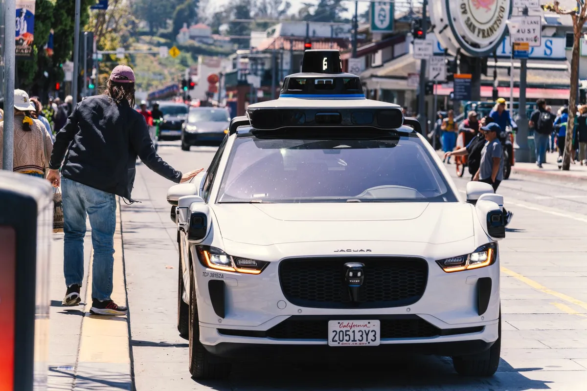
Illuminating the Road Ahead The development of Level 4 autonomous vehicles has been a long-standing goal in the automotive industry. To achieve this level of autonomy, vehicles must be able to navigate complex environments without human intervention. Two key technologies that have emerged as crucial components in this pursuit are LiDAR (Light Detection and Ranging) and computer vision. In this article, we will explore the integration of LiDAR and computer vision in Level 4 autonomy, discussing the benefits and challenges of this fusion. The Role of LiDAR in Autonomous Vehicles LiDAR is a remote sensing technology that uses laser light to measure distances and create high-resolution 3D maps of the environment. In autonomous vehicles, LiDAR is used to detect and track objects, such as other cars, pedestrians, and road features. Its high accuracy and resolution make it an ideal technology for detecting obstacles and navigating complex environments. import numpy as npdef lidar_point_cloud_processing(points): # Process LiDAR point cloud data points = np.array(points) # Filter out points with low reflectance values points = points[points[:, 3] > 0.5] return pointsThe Role of Computer Vision in Autonomous Vehicles Computer vision is a field of artificial intelligence that enables computers to interpret and understand visual data from images and videos. In autonomous vehicles, computer vision is used to detect and classify objects, such as traffic lights, pedestrians, and lane markings. Its ability to understand visual context makes it an ideal technology for navigating complex environments. import cv2def computer_vision_image_processing(image): # Process computer vision image data image = cv2.imread(image) # Apply object detection algorithm objects = cv2.detectObjects(image) return objectsFusing LiDAR and Computer Vision The integration of LiDAR and computer vision is a crucial component of Level 4 autonomy. By combining the high-resolution 3D mapping capabilities of LiDAR with the visual context understanding of computer vision, autonomous vehicles can navigate complex environments with greater accuracy and reliability. import numpy as np import cv2def fuse_lidar_and_computer_vision(lidar_points, image): # Fuse LiDAR and computer vision data lidar_points = lidar_point_cloud_processing(lidar_points) objects = computer_vision_image_processing(image) # Combine LiDAR points and computer vision objects fused_data = np.concatenate((lidar_points, objects)) return fused_dataBenefits of Fusing LiDAR and Computer Vision The integration of LiDAR and computer vision offers several benefits, including:Improved accuracy: By combining the high-resolution 3D mapping capabilities of LiDAR with the visual context understanding of computer vision, autonomous vehicles can navigate complex environments with greater accuracy and reliability. Enhanced robustness: The fusion of LiDAR and computer vision data can provide a more robust and reliable perception system, reducing the impact of sensor noise and failures. Increased flexibility: The integration of LiDAR and computer vision can enable autonomous vehicles to navigate a wider range of environments and scenarios.Challenges of Fusing LiDAR and Computer Vision The integration of LiDAR and computer vision also presents several challenges, including:Sensor calibration: The calibration of LiDAR and computer vision sensors can be a complex and time-consuming process, requiring careful alignment and synchronization of the sensors. Data fusion: The fusion of LiDAR and computer vision data can be a challenging task, requiring the development of sophisticated algorithms and techniques to combine the data from the different sensors. Computational complexity: The processing of LiDAR and computer vision data can be computationally intensive, requiring significant computational resources and power.Real-World Applications The integration of LiDAR and computer vision has several real-world applications, including:Autonomous vehicles: The fusion of LiDAR and computer vision is a crucial component of Level 4 autonomy, enabling autonomous vehicles to navigate complex environments with greater accuracy and reliability. Robotics: The integration of LiDAR and computer vision can enable robots to navigate and interact with their environment in a more robust and reliable way. Smart cities: The fusion of LiDAR and computer vision can enable smart cities to monitor and manage their infrastructure and services in a more efficient and effective way.Conclusion: A New Era of Autonomy The integration of LiDAR and computer vision is a crucial component of Level 4 autonomy, enabling autonomous vehicles to navigate complex environments with greater accuracy and reliability. While there are challenges to be addressed, the benefits of this fusion are clear, and its potential applications are vast. As the technology continues to evolve and improve, we can expect to see a new era of autonomy emerge, transforming the way we live and work. #AI #AutonomousVehicles #LiDAR #ComputerVision Related InsightsDecentralizing the Ownership of Digital Networks: Web3 Social Graphs Taming the Hallucinations: An In-Depth Analysis of Retrieval-Augmented Generation (RAG) Architectures Convergence of Robotics and Deep Learning: A New Frontier{ "@context": "https://schema.org", "@type": "FAQPage", "mainEntity": [ { "@type": "Question", "name": "What is the main focus of Fusing the Senses: The Integration of LiDAR and Computer Vision in Level 4 Autonomy?", "acceptedAnswer": { "@type": "Answer", "text": "A deep dive into the integration of LiDAR and computer vision in Level 4 autonomy, exploring the benefits and challenges of this fusion." } }, { "@type": "Question", "name": "Who authored the comprehensive guide on Fusing the Senses: The Integration of LiDAR and Computer Vision in Level 4 Autonomy?", "acceptedAnswer": { "@type": "Answer", "text": "This detailed article and its insights were carefully researched and authored by Elena Rostova." } }, { "@type": "Question", "name": "Where can I find more related content about Technology?", "acceptedAnswer": { "@type": "Answer", "text": "You can explore more articles, detailed reviews, and similar insights by browsing the Related Insights section at the bottom of this article or visiting our dedicated Technology category page." } } ] }
-
 Eleanor Sterling
 - 13 Jul, 2026 09:11
The Death of Single-Modality AI: How Multi-Sensory Architectures and Embodied Models are Redefining Cognitive Computing
For the past half-decade, the machine learning landscape has been dominated by a singular obsession: scaling the text-based transformer. From GPT-3 to the latest iterations of open-weights behemoths like Llama 3, the industry has pushed the limits of auto-regressive next-token prediction over textual corpora. Yet, text is a lossy, low-bandwidth abstraction of human knowledge. The real world is continuous, spatial, temporal, auditory, and kinetic. If we limit artificial intelligence to the linguistic domain, we sentence it to a perpetual cave of shadows, processing symbols without direct physical grounding. The paradigm has officially broken. We are witnessing the meteoric rise of true Multimodal Large Language Models (MLLMs) and Vision-Language-Action (VLA) systems. This technical evolution does not simply append an image encoder to an LLM; it structurally unifies disparate sensory inputs—video, high-fidelity audio, raw waveforms, spatial point clouds, thermal signatures, and robotic joint telemetry—into unified, high-dimensional latent spaces. This article explores the deep engineering mechanics behind this multi-sensory revolution. We will dissect the mathematical formalisms of cross-modal alignment, analyze spatiotemporal tokenization in Video-LLMs, unpack the tokenization of kinetic action in embodied AI, explore direct audio-to-audio neural architectures, and look at the systems-level infrastructure required to serve these complex, multi-headed models at scale.1. Cross-Modal Alignment and the Geometry of Unified Latent Spaces At the core of any multimodal system lies a fundamental mathematical problem: how do we project data from wildly different topological manifolds (e.g., a 1D audio waveform, a 2D spatial pixel grid, and discrete text tokens) into a shared geometric space where semantically equivalent concepts reside in close proximity? Historically, models like CLIP (Contrastive Language-Image Pre-training) achieved this using dual-encoder architectures optimized via InfoNCE loss. However, dual contrastive learning only aligns pairs. The modern frontier, pioneered by architectures like Meta's ImageBind (CVPR 2023), utilizes a hub-and-spoke model where a single modality (typically images) acts as the central binding medium. By aligning text, audio, depth, thermal, and IMU (inertial measurement unit) data to image embeddings, all modalities inherit alignment with one another without requiring explicit pairwise training data. Mathematically, let $x_i^I$ be an image representation and $x_i^M$ be a representation in another modality $M$ (e.g., audio). The projection matrices $W_I$ and $W_M$ map these representations into a shared $d$-dimensional vector space. The contrastive loss for a batch of size $N$ is defined as: $$\mathcal{L}{I, M} = -\frac{1}{N} \sum{i=1}^N \log \frac{\exp(\cos(W_I x_i^I, W_M x_i^M) / \tau)}{\sum_{j=1}^N \exp(\cos(W_I x_i^I, W_M x_j^M) / \tau)}$$ where $\tau$ is a learnable temperature parameter and $\cos(u, v) = \frac{u \cdot v}{|u| |v|}$. To feed these aligned embeddings into an auto-regressive decoder, we utilize linear projection layers or multi-head cross-attention bottlenecks (such as the Perceiver Resampler in Flamingo). This projects variable-length visual or auditory tokens into a fixed-sequence prefix that the causal transformer can ingest alongside textual embeddings.Below is a PyTorch implementation of a multi-modal projection bottleneck that aligns audio and visual feature sequences into a unified dimension suitable for insertion as soft-prompts into a decoder LLM: import torch import torch.nn as nn import torch.nn.functional as Fclass CrossModalProjectionBridge(nn.Module): def __init__(self, visual_dim: int, audio_dim: int, joint_dim: int, num_query_tokens: int): super().__init__() self.num_query_tokens = num_query_tokens self.joint_dim = joint_dim # Projection layers to align input dims to a shared space self.visual_proj = nn.Linear(visual_dim, joint_dim) self.audio_proj = nn.Linear(audio_dim, joint_dim) # Learnable query embeddings to compress variable length sequences self.query_tokens = nn.Parameter(torch.randn(1, num_query_tokens, joint_dim)) # Cross-attention block to pool representations self.cross_attention = nn.MultiheadAttention(embed_dim=joint_dim, num_heads=8, batch_first=True) self.layer_norm = nn.LayerNorm(joint_dim) self.ffn = nn.Sequential( nn.Linear(joint_dim, joint_dim * 4), nn.GELU(), nn.Linear(joint_dim * 4, joint_dim) ) def forward(self, visual_feats: torch.Tensor, audio_feats: torch.Tensor) -> torch.Tensor: # visual_feats: [batch, seq_v, visual_dim] # audio_feats: [batch, seq_a, audio_dim] batch_size = visual_feats.size(0) # Project to joint dimension v_proj = self.visual_proj(visual_feats) # [batch, seq_v, joint_dim] a_proj = self.audio_proj(audio_feats) # [batch, seq_a, joint_dim] # Concatenate multimodal context along the sequence dimension multimodal_context = torch.cat([v_proj, a_proj], dim=1) # [batch, seq_v + seq_a, joint_dim] # Expand query tokens to match batch size queries = self.query_tokens.expand(batch_size, -1, -1) # [batch, num_query, joint_dim] # Perform Cross-Attention: queries attend to key-values from multimodal context attn_out, _ = self.cross_attention( query=queries, key=multimodal_context, value=multimodal_context ) # Residual and FFN normalization pass x = self.layer_norm(queries + attn_out) out = self.layer_norm(x + self.ffn(x)) return out # Output shape: [batch, num_query, joint_dim]2. Video-LLMs and Spatiotemporal Tokenization Pipelines Moving from static images to dynamic video introduces a massive computational hurdle: the quadratic complexity of self-attention. A 10-second video at 30 frames per second contains 300 discrete images. If we tokenize each frame using a standard Vision Transformer (ViT) patch size of $14 \times 14$, we yield 256 tokens per frame, culminating in over 76,000 tokens for a short clip. To bypass this scalability wall, models like Video-LLaVA and LLaVA-NeXT employ spatial-temporal token pooling and causal spatio-temporal attention masks. Rather than passing all spatial tokens across all time slices, temporal modeling is achieved by applying 3D convolutions (like those in I3D networks) or by decoupling spatial attention (intra-frame) and temporal attention (inter-frame). Another breakthrough architecture is the Temporal Perceiver Resampler. It compresses temporal frames down to a fixed set of sequence slots by utilizing cross-attention over time vectors, allowing models to process hours of video footage within a reasonable context window. Furthermore, positional embeddings must be extended from 1D sequence markers to 3D grid indexes: $$PE_{(pos, 2i)} = \sin\left(\frac{pos}{10000^{2i/d}}\right), \quad PE_{(pos, 2i+1)} = \cos\left(\frac{pos}{10000^{2i/d}}\right)$$ where $pos$ is separately computed for the spatial $X$, $Y$ axes and the temporal $T$ axis, before being concatenated or added together. This spatial-temporal tracking allows the LLM decoder to localize actions precisely in time ("At 02:14, the user dropped the glass") and space ("The object on the far left shelf is moving"). import torch import torch.nn as nnclass SpatioTemporalTokenPooler(nn.Module): """ Compresses spatio-temporal tokens from a video stream. Input shape: [batch, temporal_frames, spatial_tokens, channels] Output shape: [batch, target_frames, compressed_tokens, channels] """ def __init__(self, channels: int, temporal_compress_ratio: int = 2, spatial_compress_ratio: int = 4): super().__init__() self.temp_pool = nn.AvgPool2d(kernel_size=(temporal_compress_ratio, 1), stride=(temporal_compress_ratio, 1)) # Spatial compression via a 2D convolution over the spatial grid self.spatial_downsample = nn.Conv2d( in_channels=channels, out_channels=channels, kernel_size=spatial_compress_ratio, stride=spatial_compress_ratio ) self.layer_norm = nn.LayerNorm(channels) def forward(self, x: torch.Tensor) -> torch.Tensor: # x shape: [B, T, S, C] where S is assumed to be a flattened square spatial grid (e.g., 256 = 16x16) batch_size, T, S, C = x.shape grid_size = int(S ** 0.5) # Reshape to perform temporal pooling: [B, C, T, S] x = x.permute(0, 3, T, S) x = self.temp_pool(x) # [B, C, T_compressed, S] new_T = x.size(2) # Reshape to perform spatial downsampling: [B * T_compressed, C, H, W] x = x.permute(0, 2, 1, 3).reshape(batch_size * new_T, C, grid_size, grid_size) x = self.spatial_downsample(x) # [B * T_compressed, C, H_new, W_new] # Reshape back to sequence form _, C_out, H_new, W_new = x.shape x = x.view(batch_size, new_T, C_out, H_new * W_new) x = x.permute(0, 1, 3, 2) # [B, T_compressed, S_compressed, C] return self.layer_norm(x)3. Embodied AI: Bridging Vision, Language, and Robotic Action One of the most consequential shifts in the AI paradigm is the transition from observer AI to agentic, physical AI. Pioneered by Google DeepMind’s RT-2 (Robotics Transformer 2) and the open-source Open X-Embodiment dataset, Vision-Language-Action (VLA) models treat robotic actions as another sequence of tokens. In a VLA model, the input consists of visual feedback from robot cameras, current joint state feedback, and a natural language instruction (e.g., "Pick up the blue marker and place it in the red bin"). The output is not merely a textual response, but a sequence of action tokens that represent control vectors for a robotic manipulator. Typically, robotic control commands are discretized into bins. A standard action vector consists of changes in spatial position ($\Delta x, \Delta y, \Delta z$), rotation ($\Delta \text{roll}, \Delta \text{pitch}, \Delta \text{yaw}$), and the state of the end-effector/gripper (open/close percentage). If we divide each dimension into 256 discrete bins, we can map these numbers directly to special token IDs in our vocabulary (e.g., tokens <action_val_112>, <action_val_45>).The model is trained auto-regressively: $$P(\text{Action} \mid \text{Vision}, \text{Text}) = \prod_{i=1}^M P(a_i \mid a_{<i}, V, T)$$ This enables the same transformer backbone that writes poetry to output precise kinematic commands, leveraging its deep world-model understanding of physics, object relationships, and reasoning directly to motor outputs. Below is an illustration of an end-to-end inference step mapping raw visual tokens and instructions into robotic control signals: import numpy as npclass ActionTokenDecoder: """ Decodes discrete LLM output tokens back into continuous physical robot trajectories. """ def __init__(self, num_bins: int = 256, action_ranges: dict = None): self.num_bins = num_bins # Default physical limits for manipulator translation (meters) and rotation (radians) self.ranges = action_ranges or { 'x': (-1.0, 1.0), 'y': (-1.0, 1.0), 'z': (-1.0, 1.0), 'roll': (-np.pi, np.pi), 'pitch': (-np.pi, np.pi), 'yaw': (-np.pi, np.pi), 'gripper': (0.0, 1.0) } self.keys = ['x', 'y', 'z', 'roll', 'pitch', 'yaw', 'gripper'] def decode_token_to_value(self, bin_index: int, val_range: tuple) -> float: # Convert index in range [0, 255] to a continuous float min_val, max_val = val_range normalized_val = bin_index / (self.num_bins - 1) return min_val + normalized_val * (max_val - min_val) def parse_action_sequence(self, token_indices: list) -> dict: """ Expects a list of 7 integers corresponding to action tokens. """ assert len(token_indices) == len(self.keys), f"Expected 7 action tokens, got {len(token_indices)}" action_dict = {} for idx, key in enumerate(self.keys): bin_index = token_indices[idx] # Ensure index falls within bin limitations clamped_bin = max(0, min(bin_index, self.num_bins - 1)) action_dict[key] = self.decode_token_to_value(clamped_bin, self.ranges[key]) return action_dict# Example Usage decoder = ActionTokenDecoder() # Dummy model predicted token IDs mapped to discrete bins: [128, 64, 192, 128, 128, 96, 255] predicted_action_bins = [128, 64, 192, 128, 128, 96, 255] kinematic_command = decoder.parse_action_sequence(predicted_action_bins) print("Physical kinematics target values:", kinematic_command)4. Auditory Cognition: End-to-End Speech-to-Speech and Acoustic Embedding For years, speech interface pipelines were clunky cascades:Automatic Speech Recognition (ASR): Audio Waveform $\to$ Text (via Whisper/Conformer) Text Processing: Text $\to$ Text response (via LLM) Text-to-Speech (TTS): Text response $\to$ Output Waveform (via Tacotron/VALL-E)This multi-hop approach suffers from high latency and completely strips voice communication of its emotional, tonal, and non-verbal nuances (sarcasm, dynamic pauses, breathiness, background noise). Modern native speech-to-speech architectures (exemplified by GPT-4o and Meta’s SeamlessM4T) collapse this pipeline into a single, unified, end-to-end model. This is achieved by utilizing neural audio codecs such as EnCodec or Descript Audio Codec (DAC). These neural codecs compress raw continuous audio waveforms down into discrete codes using Vector Quantized Variational Autoencoders (VQ-VAE) or Residual Vector Quantization (RVQ).The continuous audio is converted into several streams of discrete acoustic codes (quantized channels), which are flattened and interleaved into the transformer’s core tokenizer. Audio generation becomes identical to text generation: the model outputs acoustic tokens, which are fed directly to the decoder portion of the neural codec to synthesize high-fidelity, expressive, low-latency audio waveforms. The objective function remains standard cross-entropy calculated over the quantized acoustic sequence tokens: $$\mathcal{L} = -\sum_{t=1}^T \log P(u_t \mid u_{<t}, H_{audio})$$ where $u_t$ is the target acoustic token at sequence step $t$, and $H_{audio}$ represents the encoded auditory condition vector.5. Production Architecture: Orchestrating Ultra-Low Latency Multimodal Pipelines Serving models that dynamically process video, audio, and text at scale requires complete re-engineering of the typical LLM serving stack (vLLM, Hugging Face TGI). When serving a multimodal system, memory management of the KV cache becomes an existential threat to high-throughput operations. While text token embeddings are tiny, a single high-resolution image processed through a ViT can generate 576 or more embeddings. Storing these embeddings across layers in the Key-Value (KV) cache of the transformer rapidly exhausts the H100 or A100 GPU’s High Bandwidth Memory (HBM). To solve this, modern inference engines apply Prefix Caching and FlashAttention-style Multi-Modal Kernels. If a user is conversing about a 10-minute video, the video tokens are loaded, processed, and locked in the KV cache as a static system prompt prefix. Subsequent user text turns only reference this pre-computed, immutable prefix cache, avoiding redundant re-evaluations. Furthermore, inference engines must handle dynamic input routing, sending heavy vision processing workloads to dedicated vision pipeline backends before routing projection matrices to the core tensor-parallel autoregressive engine. # docker-compose.prod.yml # Production deployment configuration for a Multi-Modal inference cluster version: '3.8'services: triton-inference-server: image: nvcr.io/nvidia/tritonserver:26.01-py3 container_name: multimodal_triton_server shm_size: '16gb' deploy: resources: reservations: devices: - driver: nvidia count: all capabilities: [gpu] environment: - TRITON_SERVER_MODEL_REPOSITORY=/models - CUDA_VISIBLE_DEVICES=0,1,2,3 ports: - "8000:8000" # HTTP endpoint - "8001:8001" # gRPC endpoint - "8002:8002" # Metrics endpoint volumes: - ./model_repository:/models command: ["tritonserver", "--model-repository=/models", "--log-verbose=1", "--pinned-memory-pool-byte-size=268435456"] restart: always vllm-multimodal-engine: image: vllm/vllm-openai:latest container_name: vllm_multimodal_api environment: - CUDA_VISIBLE_DEVICES=4,5,6,7 - NCCL_DEBUG=INFO ports: - "8005:8000" volumes: - ~/.cache/huggingface:/root/.cache/huggingface deploy: resources: reservations: devices: - driver: nvidia count: 4 capabilities: [gpu] command: > python3 -m vllm.entrypoints.openai.api_server --model Qwen/Qwen2-VL-7B-Instruct --tensor-parallel-size 4 --trust-remote-code --max-model-len 32768 --gpu-memory-utilization 0.90 --max-num-seqs 256 restart: alwaysMultimodal Paradigms: A Structural Comparison To understand the trade-offs between different multimodal architectures, we can analyze the structures of early-fusion, late-fusion, and multi-encoder alignment models.Architectural Metric Early Fusion (Unified Tokenization) Late Fusion (Ensemble/Decision level) Cross-Attention / Bottleneck Alignment (Flamingo/BLIP-2) Unified Latent Projection (ImageBind)Data Ingestion Raw tokens interleaved at input layer Independent encoders, combined at logits Separate visual encoder, mapped via cross-attention Multi-headed projection to centralized hub spaceInference Latency High (large context sequence overhead) Minimal (parallel independent passes) Medium (attention bottlenecks add overhead) Low to Medium (efficient multi-sensor retrieval)Modal Interaction Direct (full self-attention across modalities) None (isolated until final layer) Medium (queries attend to frozen sensory keys) High (shared geometric similarity metrics)Primary Use Cases GPT-4o, Native Audio/Video LLMs Multi-sensor classification ensembles LLaVA, Video-LLaVA, Visual Question Answering Zero-shot multi-sensory retrieval, cross-modal searchThe table above demonstrates that while Early Fusion architectures provide the deepest level of multi-sensory understanding by allowing every modality token to pay direct attention to every other token, they suffer from high inference latency and rapid context-window exhaustion. Conversely, Cross-Attention Bottleneck models strike a practical production balance, making them highly popular for real-world visual-reasoning applications.Conclusion: The Horizon of Generalist Physical Agents We are moving past the era where artificial intelligence is mere software operating behind glass screens. The unification of speech, vision, dynamic temporal context, and motor outputs is coalescing into a single, cohesive framework: the Generalist Physical Agent. By building unified embeddings that span the entirety of physical experience, we are laying the groundwork for systems that learn from observation, follow complex environmental commands, and dynamically manipulate physical environments with human-like spatial precision. The future of machine intelligence is not linguistic; it is multi-sensory. The models that will define the next decade of human history are those that can see, hear, speak, touch, and move across our physical reality.#AI #MachineLearning #Robotics #ComputerVision #DeepLearning Related InsightsThe Thermodynamic Horizon: Decoding the Convergence of AI-Driven Fusion and Kinetic Energy Grids The Digital Scalpel: Architecting High-Fidelity Haptic Feedback in Robotic Surgery Simulation Unlocking the Quantum Epoch: How QML Will Revolutionize Data Science and AI as We Know It{ "@context": "https://schema.org", "@type": "FAQPage", "mainEntity": [ { "@type": "Question", "name": "What is the main focus of The Death of Single-Modality AI: How Multi-Sensory Architectures and Embodied Models are Redefining Cognitive Computing?", "acceptedAnswer": { "@type": "Answer", "text": "An in-depth technical analysis of the architectural shift from unimodal LLMs to unified, multi-sensory AI models integrating video, audio, telemetry, and robotic action tokens." } }, { "@type": "Question", "name": "Who authored the comprehensive guide on The Death of Single-Modality AI: How Multi-Sensory Architectures and Embodied Models are Redefining Cognitive Computing?", "acceptedAnswer": { "@type": "Answer", "text": "This detailed article and its insights were carefully researched and authored by Eleanor Sterling." } }, { "@type": "Question", "name": "Where can I find more related content about Technology?", "acceptedAnswer": { "@type": "Answer", "text": "You can explore more articles, detailed reviews, and similar insights by browsing the Related Insights section at the bottom of this article or visiting our dedicated Technology category page." } } ] }