Showing Posts From
Quantummachinelearning

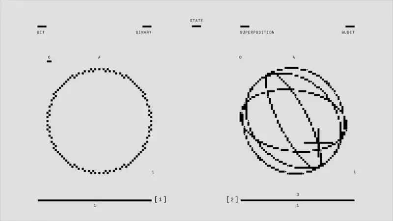
Navigating the Quantum Frontier of Artificial Intelligence As a senior software engineer and AI researcher, I have watched deep learning scale to unimaginable heights. We have built multi-billion parameter transformers, colossal video understanding pipelines, and intricate multimodal architectures that can reason, parse code, and synthesize media. Yet, we are rapidly hitting the wall of classical compute limits. Moore's Law has plateaued, thermal dissipation remains a brutal enemy, and the energy footprint of training foundational models is starting to challenge planetary resource thresholds. Enter Quantum Machine Learning (QML), a paradigm that promises to fundamentally disrupt how we process information, shift the boundaries of computational complexity, and unlock optimization landscapes previously locked behind exponential walls.The marriage of quantum mechanics and machine learning is not merely an academic exercise; it is an engineering necessity for the next century of intelligence. Classical computers process information in deterministic bits—zeros and ones. Quantum computers leverage qubits, harnessing the bizarre, counter-intuitive properties of quantum mechanics: superposition, entanglement, and interference. When we project machine learning tasks—such as high-dimensional matrix inversions, kernel estimations, and combinatorial optimizations—onto these quantum states, entire algorithmic complexities transform. Where classical processors require $\mathcal{O}(2^n)$ steps to navigate complex state spaces, certain quantum algorithms can evaluate global configurations simultaneously. However, bridging the gap between theoretical quantum advantage and production-ready machine learning workflows requires immense architectural rigor. We cannot simply drop a classical neural network onto a quantum processor. We must rethink representation learning, gradient computation, and loss optimization from the ground up. In this deep dive, we will explore the architectural principles of QML, analyze how cutting-edge self-supervised frameworks and geometric deep learning concepts parallel quantum structural challenges, and implement production-grade code leveraging modern hybrid quantum-classical frameworks. Deconstructing Hybrid Quantum-Classical Architectures The contemporary era of quantum computing is defined by the Noisy Intermediate-Scale Quantum (NISQ) regime. Current quantum processors feature limited qubit counts and are susceptible to decoherence and gate errors. Consequently, pure quantum machine learning models are presently impractical for industrial workloads. Instead, the industry relies on hybrid quantum-classical architectures, specifically Parameterized Quantum Circuits (PQCs), often styled as quantum neural networks (QNNs). In a hybrid pipeline, a classical system handles data preprocessing, feature extraction, and gradient descent optimization, while the quantum processing unit (QPU) acts as a specialized coprocessor. The QPU evaluates parameterized unitary operations that transform input states into measurement outcomes. These measurements serve as expectations that feed directly into classical loss functions. +-----------------------------------------------------------------+ | CLASSICAL HOST SYSTEM | | [Data Ingestion] ---> [Feature Encoding] ---> [Optimizer] | +---------------------------------------|-------------------------+ | Parameters (theta) v +---------------------------------------+-------------------------+ | QUANTUM PROCESSING UNIT (QPU) | | [State Prep] ---> [Parameterized Gates (U(theta))] ---> [Measure]| +---------------------------------------|-------------------------+ | Expectation Values v +---------------------------------------+-------------------------+ | CLASSICAL HOST SYSTEM | | [Loss Calculation] <--- [Backpropagation / Parameter Update] | +-----------------------------------------------------------------+The mathematical foundation governing these circuits relies on the parameter-shift rule, an analytical method for computing gradients of quantum circuits without relying on numerical finite-difference approximations. Given an expectation value $E(\theta)$ of an observable $H$ with respect to a state prepared by a parameterized unitary $U(\theta) = \exp(-i \theta P / 2)$ generated by a Pauli operator $P$, the exact derivative with respect to parameter $\theta$ is expressed as: $$\frac{\partial E(\theta)}{\partial \theta} = \frac{E\left(\theta + \frac{\pi}{2}\right) - E\left(\theta - \frac{\pi}{2}\right)}{2}$$ This elegance allows classical optimizers like Adam or L-BFGS to tune quantum circuit parameters seamlessly. Yet, practitioners must navigate the notorious barren plateau problem. As quantum circuits grow deeper and wider, the variance of their cost function gradients vanishes exponentially toward zero, rendering training nearly impossible. Mitigating barren plateaus requires careful ansatz design, localized cost functions, and shallow circuit topologies that mirror the inductive biases found in advanced classical paradigms. Parallels in Structural Evolution: From Self-Distillation to Curvature Guidance To understand how quantum machine learning will scale, we can examine recent breakthroughs in classical deep learning architectures that grapple with high-dimensional complexity, data scarcity, and representation bottlenecks. Recent arXiv literature showcases architectural innovations that offer profound methodological parallels to quantum algorithmic design. Consider the framework of Temporal Self-Distillation (S$^3$T) designed for continuous video state tracking. S$^3$T treats temporal sampling density as privileged information, using a dense-view teacher network to guide a sparse-view student model via self-distillation without human labels or reward signals. In quantum computing, a analogous compression challenge exists: mapping massive, high-dimensional Hilbert spaces down to manageable, interpretable classical measurements without losing global structural fidelity. Both domains rely on internal self-consistency—leveraging richer structural views (whether dense video frames or multi-qubit entanglement profiles) to train efficient, low-overhead inference engines.Similarly, look at TokenMatch, a transformer-based model for 3D shape correspondence that utilizes curvature-guided tokenisation. Meshes are adaptively tokenized into patches based on local shape curvature, allowing the transformer to learn geometry-specific descriptors efficiently. In quantum algorithm design, spatial and topological awareness is equally critical. Graph neural networks and quantum kernel methods must encode complex molecular structures or high-dimensional financial graphs into quantum states using amplitude encoding or Hamiltonian simulation. By utilizing geometric priors—such as curvature-guided tokenisation or equivariant graph layers—we can drastically reduce the dimensionality of the quantum state space required to represent complex physical systems. Let us review a production-grade Python script utilizing PennyLane and PyTorch to construct a hybrid quantum-classical neural network layer. This script initializes a quantum device, constructs a parameterized quantum circuit with rotational and entangling gates, and embeds it directly into a PyTorch module for end-to-end gradient descent optimization. import torch import torch.nn as nn import pennylane as qml# Configure the quantum device with 4 qubits n_qubits = 4 dev = qml.device("default.qubit", wires=n_qubits)@qml.qnode(dev, interface="torch", diff_method="parameter-shift") def quantum_circuit(inputs, weights): """ Parameterized Quantum Circuit acting as a quantum layer. Args: inputs (torch.Tensor): Classical input features encoded via angle embedding. weights (torch.Tensor): Trainable weights for the variational circuit. """ # Encode classical data into quantum states using angle embedding qml.AngleEmbedding(inputs, wires=range(n_qubits), rotation='Y') # Apply layers of parameterized rotations and entanglement qml.StronglyEntanglingLayers(weights, wires=range(n_qubits)) # Return expectation values for all qubits along the Z axis return [qml.expval(qml.PauliZ(i)) for i in range(n_qubits)]class HybridQuantumClassicalModel(nn.Module): """ Hybrid neural network combining classical linear layers with a QPU layer. """ def __init__(self, input_dim: int, n_layers: int, output_dim: int): super(HybridQuantumClassicalModel, self).__init__() # Classical preprocessing network self.pre_net = nn.Sequential( nn.Linear(input_dim, n_qubits), nn.Tanh() ) # Define shape for StronglyEntanglingLayers weights: (n_layers, n_qubits, 3) weight_shapes = {"weights": (n_layers, n_qubits, 3)} # Wrap the PennyLane QNode as a PyTorch Module layer self.q_layer = qml.qnn.TorchLayer(quantum_circuit, weight_shapes) # Classical post-processing network self.post_net = nn.Sequential( nn.Linear(n_qubits, 16), nn.ReLU(), nn.Linear(16, output_dim) ) def forward(self, x: torch.Tensor) -> torch.Tensor: # Step 1: Classical dimensionality reduction / feature mapping x = self.pre_net(x) # Step 2: Scale inputs to appropriate angular range [0, pi] x = torch.sigmoid(x) * torch.pi # Step 3: Pass through the quantum variational circuit x = self.q_layer(x) # Step 4: Final classical inference layer out = self.post_net(x) return out# Instantiation and verification of the hybrid architecture if __name__ == "__main__": model = HybridQuantumClassicalModel(input_dim=8, n_layers=2, output_dim=2) sample_input = torch.randn(32, 8) # Batch of 32 samples, 8 features each predictions = model(sample_input) print(f"Hybrid QML Output Tensor Shape: {predictions.shape}")Quantum Kernels and Support Vector Machines in High-Dimensional Spaces One of the most mathematically rigorous and industrially promising applications of QML is the Quantum Kernel Method. Classical kernel methods, such as Support Vector Machines (SVMs), compute inner products between data points in a high-dimensional feature space using kernel functions $\mathcal{K}(x, x') = \langle \phi(x), \phi(x') \rangle$. This trick allows linear algorithms to discover complex, non-linear decision boundaries. However, designing feature maps $\phi(x)$ that project classical data into spaces where linear separation is trivial becomes computationally intractable as dimensionality explodes. Quantum computers excel precisely at this task. By defining a quantum feature map $U(\phi(x))$ that prepares a quantum state $|\phi(x)\rangle = U(\phi(x))|0\rangle$, the overlap between two quantum states naturally computes the kernel value via the fidelity measurement: $$\mathcal{K}(x, x') = |\langle 0 | U^\dagger(\phi(x)) U(\phi(x')) | 0 \rangle|^2$$ This inner product can be measured directly on a quantum processor using a SWAP test or an overlap test. The profound implication here is that quantum kernels can access feature Hilbert spaces of dimension $2^n$ (where $n$ is the number of qubits) that are entirely classically unsimulatable. To orchestrate quantum kernel training in a production environment, machine learning engineers deploy containerized orchestration pipelines. Below is a production-ready Docker Compose configuration designed to spin up a distributed QML training cluster, coupling a Jupyter lab interface for algorithm prototyping with a dedicated Ray cluster for parallelizing quantum circuit executions across simulated or physical QPU workers. version: '3.8'services: qml-jupyter: image: qml/research-workspace:latest container_name: qml_jupyter_lab ports: - "8888:8888" environment: - JUPYTER_ENABLE_LAB=yes - QISKIT_IBM_TOKEN=${QISKIT_IBM_TOKEN} volumes: - ./notebooks:/workspace/notebooks - ./src:/workspace/src deploy: resources: reservations: devices: - driver: nvidia count: 1 capabilities: [gpu] networks: - qml-net ray-head: image: rayproject/ray:latest-gpu container_name: ray_cluster_head command: ray start --head --node-ip-address=0.0.0.0 --port=6379 --block ports: - "6379:6379" - "8265:8265" # Ray Dashboard networks: - qml-net ray-worker: image: rayproject/ray:latest-gpu container_name: ray_cluster_worker command: ray start --address='ray-head:6379' --block depends_on: - ray-head networks: - qml-netnetworks: qml-net: driver: bridgeMitigating Noise and Enhancing Fault Tolerance in Quantum Pipelines The primary barrier preventing widespread enterprise adoption of quantum machine learning is quantum noise. Qubits are exceptionally fragile. Environmental magnetic fluctuations, thermal noise, and imperfect gate calibrations induce decoherence, corrupting state vectors and introducing catastrophic errors into gradient calculations. In classical deep learning, we combat noise with dropout, weight decay, and batch normalization. In QML, we must engineer error mitigation and fault-tolerant algorithms at both the software and hardware layers. Error mitigation techniques—such as Zero-Noise Extrapolation (ZNE) and Probabilistic Error Cancellation (PEC)—allow algorithms to extract meaningful signal from noisy hardware without requiring full-scale quantum error correction (which demands millions of physical qubits per logical qubit). ZNE operates by intentionally stretching the noise level of a quantum circuit (e.g., by scaling pulse durations or repeating gates as $U \rightarrow U (U^\dagger U)^k$), measuring expectation values at multiple noise scales, and mathematically extrapolating back to the zero-noise limit. Furthermore, variational quantum algorithms exhibit a degree of inherent noise resilience. Because PQCs are optimized iteratively via classical feedback loops, the classical optimizer can occasionally learn to steer around systematic hardware biases or calibration drift, effectively treating hardware imperfections as part of the operational loss landscape.As we transition toward fault-tolerant quantum computing (FTQC), machine learning engineers will begin integrating quantum error correction (QEC) codes directly into data pipelines. Surface codes and color codes will protect superposition states, ensuring that deep quantum circuits can execute thousands of consecutive gates without succumbing to decoherence. This technological inflection point will unleash the true potential of Quantum Generative Adversarial Networks (QGANs) and quantum reinforcement learning agents, solving combinatorial optimization and drug discovery problems at speeds that render classical supercomputers obsolete. Engineering the Future: Integration and Scalability Challenges Deploying Quantum Machine Learning models into enterprise production pipelines introduces unique software engineering challenges. Unlike classical models that rely on standard REST or gRPC microservices running on CPU/GPU clusters, QML inference requires asynchronous request routing to specialized quantum hardware providers (such as IBM Quantum, IonQ, or Rigetti) or local high-performance state-vector simulators. Latency is a critical bottleneck. Network round-trip times to cloud-hosted QPUs, combined with queue wait times for quantum job scheduling, make real-time inference (such as sub-millisecond autonomous vehicle control) currently unfeasible via pure cloud quantum access. Consequently, production architectures must implement intelligent fallback mechanisms. When QPU latency spikes or quantum jobs time out, the system must seamlessly degrade to classical surrogate models—distilled neural networks trained to approximate the quantum circuit's behavior with minimal loss in accuracy. As an AI researcher, I advise engineering teams to adopt a modular design pattern. Separate your feature encoding logic, quantum circuit definitions, and classical optimization loops into decoupled microservices. Utilize asynchronous task queues like Celery or Apache Kafka to manage quantum job payloads, and maintain robust telemetry dashboards to monitor QPU fidelity metrics, gate error rates, and classical optimizer convergence trajectories in real time. Concluding Perspectives on Quantum Acceleration Quantum Machine Learning represents the convergence of two of the most transformative technological revolutions in human history. While we currently navigate the turbulent waters of the NISQ era, the mathematical foundations, algorithmic frameworks, and hybrid architectures being developed today are laying the groundwork for a post-classical computing paradigm. By bridging quantum kernels, parameterized quantum circuits, and advanced geometric optimization techniques, we are expanding the horizons of what artificial intelligence can achieve. The journey from theoretical Hamiltonian simulation to production-grade quantum AI will require rigorous engineering, relentless innovation, and interdisciplinary mastery. The quantum future of AI is not a distant sci-fi fantasy—it is being compiled, tested, and optimized in labs and repositories across the globe right now.#QuantumComputing #MachineLearning #ArtificialIntelligence #QuantumMachineLearning #TechInnovation #DeepLearning #FutureTech Related InsightsThe Silicon Synthesis: Navigating the Future of Autonomous Agency and Labor Revolutionizing Moore's Law: The Rise of Graphene-Based Semiconductors Sustainable Tech - Part 02: Biodegradable Substrates for Circuit Boards{ "@context": "https://schema.org", "@type": "FAQPage", "mainEntity": [ { "@type": "Question", "name": "What is the main focus of Quantum Machine Learning: Speeding Up AI with Quantum Algorithms?", "acceptedAnswer": { "@type": "Answer", "text": "Explore the intersection of quantum computing and machine learning, examining how advanced algorithmic architectures revolutionize artificial intelligence." } }, { "@type": "Question", "name": "Who authored the comprehensive guide on Quantum Machine Learning: Speeding Up AI with Quantum Algorithms?", "acceptedAnswer": { "@type": "Answer", "text": "This detailed article and its insights were carefully researched and authored by Sofia Morales." } }, { "@type": "Question", "name": "Where can I find more related content about Technology?", "acceptedAnswer": { "@type": "Answer", "text": "You can explore more articles, detailed reviews, and similar insights by browsing the Related Insights section at the bottom of this article or visiting our dedicated Technology category page." } } ] }
-
 Kaan Demir
 - 13 Jul, 2026 18:56
Unlocking the Quantum Epoch: How QML Will Revolutionize Data Science and AI as We Know It
In the ever-accelerating race for computational supremacy, classical machine learning models, despite their impressive advancements, are beginning to brush against fundamental limits. As datasets burgeon in size and complexity, the computational cost of extracting meaningful insights grows exponentially. We're witnessing the rise of complex, non-linear relationships that even the most sophisticated deep learning architectures struggle to untangle efficiently. This inflection point heralds the arrival of an entirely new paradigm: Quantum Machine Learning (QML). Not merely an incremental upgrade, QML represents a profound architectural shift, leveraging the counter-intuitive yet powerful principles of quantum mechanics—superposition, entanglement, and quantum interference—to process information in ways fundamentally impossible for classical computers. This isn't speculative fiction; it's the bleeding edge of academic research transitioning rapidly into practical development. From arXiv preprints detailing novel quantum kernel methods to GitHub repositories showcasing open-source QML frameworks like Qiskit, Cirq, and PennyLane, the foundations are being laid. TechCrunch and Y Combinator reports increasingly highlight startups pushing the boundaries of quantum algorithms, attracting significant investment. QML promises to unlock unprecedented capabilities in areas ranging from drug discovery and materials science to financial modeling and advanced artificial intelligence, potentially solving problems currently intractable for even the world's most powerful supercomputers. This article will delve into the technical underpinnings, key algorithms, hybrid architectures, and the practical tools shaping this thrilling new frontier, providing a roadmap for data scientists ready to embark on the quantum journey. The Quantum Leap in Data Representation: Qubits and Feature MapsAt the core of Quantum Machine Learning lies a radical departure from classical data representation. While classical bits exist in a definite state of 0 or 1, quantum bits, or qubits, can exist in a superposition of both states simultaneously. This inherent probabilistic nature, combined with entanglement—where qubits become correlated in a way that transcends classical physics—allows for an exponential increase in the information density and processing power of a quantum system. A system of n qubits can represent 2^n states concurrently, a phenomenon that provides the quantum advantage for certain types of computations. The critical first step in applying quantum algorithms to classical machine learning problems is transforming classical data into quantum states. This is achieved through Quantum Feature Maps (QFMs). A QFM is essentially a parametrized quantum circuit that encodes classical input data points x into a high-dimensional quantum Hilbert space, typically by applying a series of quantum gates controlled by the input features. The goal is to map data in such a way that patterns and relationships that are obscure in classical space become more separable or distinguishable in the quantum space, often making linear separations possible in an exponentially larger feature space. This is analogous to the "kernel trick" in classical Support Vector Machines (SVMs), but with the potential to explore feature spaces of vastly greater dimensions. The choice of QFM is crucial, as an inappropriate mapping can lead to issues like "barren plateaus" in variational algorithms, where gradients vanish, hindering optimization. Consider a simple quantum feature map implemented using Qiskit. This map might involve applying single-qubit rotations (like R_x, R_y, R_z) and entangling gates (like CNOT) whose parameters are derived from the input data. import numpy as np from qiskit import QuantumCircuit, Aer, transpile from qiskit.opflow import StateFn, PauliSumOp from qiskit.utils import QuantumInstance from qiskit.circuit.library import ZZFeatureMap# 1. Define a classical data point (e.g., 2 features) x = np.array([0.5, 0.8])# 2. Choose a Quantum Feature Map. ZZFeatureMap is a common choice. # It encodes data using Z-rotations and ZZ-interactions. # 'reps' parameter controls the depth of the circuit (how many times the pattern repeats). feature_map = ZZFeatureMap(feature_dimension=len(x), reps=2, entanglement='linear')# 3. Bind the classical data to the feature map # The feature map will use 'x' to set its parameters. feature_map_circuit = feature_map.assign_parameters(x)# 4. Visualize the circuit (optional) # print(feature_map_circuit.decompose())# 5. Simulate the state prepared by the feature map simulator = Aer.get_backend('statevector_simulator') quantum_instance = QuantumInstance(simulator, shots=1024)# Create a job to run the circuit job = simulator.run(transpile(feature_map_circuit, simulator)) result = job.result() statevector = result.get_statevector(feature_map_circuit)print("Classical Input Data:", x) print("Quantum Feature Map Circuit Depth:", feature_map_circuit.depth()) print("Quantum State Vector (Magnitude):", np.round(np.abs(statevector), 4)) print("This state vector represents the classical data encoded in a high-dimensional quantum space.")# For a more complex application, this state could then be fed into a quantum kernel # or a variational quantum classifier.This Python snippet demonstrates how classical data x is encoded into a quantum state via a ZZFeatureMap. The resulting state vector exists in a complex Hilbert space, where distances and similarities between data points can be profoundly different from their classical counterparts. This initial encoding step is foundational, setting the stage for subsequent quantum algorithms to operate on these quantum representations of data. Quantum Enhanced Algorithms: QSVMs and QNNsLeveraging these quantum feature maps, two prominent classes of algorithms emerge in Quantum Machine Learning: Quantum Support Vector Machines (QSVMs) and Quantum Neural Networks (QNNs). These algorithms aim to harness quantum phenomena to outperform their classical counterparts, particularly in tasks involving complex, high-dimensional data. Quantum Support Vector Machines (QSVMs) are direct quantum extensions of classical SVMs. The core idea is to replace the classical kernel function, which measures the similarity between data points in a high-dimensional feature space, with a Quantum Kernel. A quantum kernel calculates the inner product between two quantum feature states, $\kappa(x_i, x_j) = |\langle\phi(x_i)|\phi(x_j)\rangle|^2$, where $\phi(x)$ is the quantum state encoded by the feature map from classical data x. This kernel value, estimated by running quantum circuits, is then fed into a classical SVM optimizer. The quantum advantage here stems from the ability of QFMs to implicitly map data into exponentially larger Hilbert spaces than classical kernels can practically achieve, potentially leading to better separation boundaries for non-linearly separable data. However, precisely estimating these kernel values can be computationally intensive and susceptible to quantum noise. Quantum Neural Networks (QNNs), often referred to as Variational Quantum Circuits (VQCs) or Parametrized Quantum Circuits (PQCs), represent a hybrid quantum-classical approach inspired by classical neural networks. A QNN consists of a parametrized quantum circuit whose gate rotation angles are trainable parameters. The circuit takes classical data (encoded via a QFM) and processes it to produce an output, often an expectation value of a specific observable. This output is then fed into a classical loss function, and a classical optimizer updates the quantum circuit's parameters based on the gradient of the loss. This iterative process, where quantum hardware performs the forward pass and classical computers handle optimization, is a hallmark of the Noisy Intermediate-Scale Quantum (NISQ) era, where full quantum error correction is not yet available. A typical QNN might look like a series of interleaved layers of single-qubit rotations and entangling gates, where the rotation angles are the variational parameters. Training these QNNs involves challenges such as barren plateaus, where the landscape of the loss function becomes extremely flat for deep circuits, making gradient-based optimization difficult. Techniques like parameter shift rules are used to calculate gradients on quantum hardware. Here's a conceptual Python example demonstrating a simple QNN (VQC) with PennyLane, showing the hybrid optimization loop: import pennylane as qml from pennylane import numpy as np from pennylane.optimize import AdamOptimizer# 1. Define the quantum device dev = qml.device("default.qubit", wires=2)# 2. Define the Parametrized Quantum Circuit (PQC / QNN) # This circuit will act as our 'quantum layer' @qml.qnode(dev) def qnn(weights, x): # Encoding layer (simple example using angles from data) qml.RY(x[0], wires=0) qml.RX(x[1], wires=1) # Variational layer (trainable parameters 'weights') qml.Rot(weights[0, 0], weights[0, 1], weights[0, 2], wires=0) qml.Rot(weights[1, 0], weights[1, 1], weights[1, 2], wires=1) qml.CZ(wires=[0, 1]) qml.Rot(weights[2, 0], weights[2, 1], weights[2, 2], wires=0) qml.Rot(weights[3, 0], weights[3, 1], weights[3, 2], wires=1) # Measurement (expectation value for classification) return qml.expval(qml.PauliZ(0))# 3. Define a classical cost function def cost(weights, X, y): predictions = [qnn(weights, x) for x in X] # Simple squared error loss return np.mean((np.array(predictions) - y)**2)# 4. Generate some dummy data for demonstration X = np.array([[0.1, 0.2], [0.3, 0.4], [0.5, 0.6], [0.7, 0.8]], requires_grad=False) y = np.array([0.0, 0.2, 0.5, 0.8], requires_grad=False) # Target outputs# 5. Initialize random weights for the QNN # Number of weights depends on the circuit architecture (4x3 rotations + 1 CZ) weights = np.random.uniform(low=-np.pi, high=np.pi, size=(4, 3), requires_grad=True)# 6. Set up the classical optimizer opt = AdamOptimizer(stepsize=0.1)# 7. Training loop (hybrid quantum-classical optimization) epochs = 50 print("Initial cost:", cost(weights, X, y))for epoch in range(epochs): weights, current_cost = opt.step_and_cost(cost, weights, X, y) if (epoch + 1) % 10 == 0: print(f"Epoch {epoch+1}, Cost: {current_cost:.4f}")print("Optimized weights:", weights) print("Final cost:", cost(weights, X, y))This example illustrates the fundamental hybrid approach: the quantum qnn function computes an output based on data and weights, and a classical AdamOptimizer iteratively adjusts these weights to minimize a cost function. This synergy between quantum and classical components is key to near-term QML applications. Hybrid Quantum-Classical Architectures for ScalabilityThe current state of quantum hardware, characterized by the NISQ (Noisy Intermediate-Scale Quantum) era, necessitates a hybrid approach to Quantum Machine Learning. Full-scale, fault-tolerant quantum computers are still years away. Therefore, for practical applications, QML algorithms often involve a delicate dance between quantum processors (QPUs) and classical computing resources. This hybrid architecture is not a temporary workaround but a fundamental paradigm for leveraging the nascent power of QPUs. In a hybrid setup, the computationally intensive parts that benefit from quantum mechanics (e.g., preparing complex quantum states, executing quantum kernels, performing specific unitary transformations) are offloaded to a QPU. Meanwhile, classical computers handle tasks like data pre-processing, post-processing, optimization of quantum circuit parameters, and overall control flow. This modular design allows researchers to tackle problems too complex for classical machines alone while circumventing the limitations of current noisy quantum hardware. Key hybrid algorithms include:Variational Quantum Eigensolver (VQE): Primarily used in quantum chemistry for finding the ground state energy of molecules. A QPU prepares an ansatz state, measures its energy, and a classical optimizer iteratively adjusts the ansatz parameters to minimize the energy. Quantum Approximate Optimization Algorithm (QAOA): Designed for combinatorial optimization problems. Similar to VQE, it uses a parametrized quantum circuit to explore solution spaces and a classical optimizer to find optimal parameters.The interaction between the classical and quantum components often involves a feedback loop:Classical Pre-processing: Prepare classical data, design the quantum circuit structure (ansatz). Data Encoding: Map classical data to quantum states on the QPU. Quantum Circuit Execution: Run the parametrized quantum circuit on the QPU. This generates quantum measurements. Classical Measurement Post-processing: Extract expectation values or probabilities from quantum measurements. Classical Optimization: Use the extracted values in a classical cost function and update the quantum circuit's parameters (e.g., gate rotation angles) using classical optimization algorithms (like Adam, L-BFGS-B). Iteration: Send the updated parameters back to the QPU for the next iteration.One of the significant challenges in these architectures is the data transfer bottleneck between classical and quantum systems, as well as managing error accumulation on noisy QPUs. Techniques like measurement error mitigation and readout error correction are crucial. Consider a conceptual Bash script that outlines a workflow for running a QML experiment, demonstrating the interplay: #!/bin/bash# This script simulates a hybrid quantum-classical workflow. # It assumes you have a Python environment set up with Qiskit/PennyLane.echo "Starting Hybrid Quantum-Classical QML Experiment..."# --- Phase 1: Classical Data Preprocessing --- echo "1. Performing classical data preprocessing..." python -c " import numpy as np # Simulate loading and cleaning data data = np.random.rand(100, 2) labels = (np.sum(data, axis=1) > 1.0).astype(int) np.save('processed_data.npy', data) np.save('processed_labels.npy', labels) print('Data preprocessed and saved to processed_data.npy and processed_labels.npy') " echo "Data preprocessing complete."# --- Phase 2: Initialize Quantum Circuit Parameters Classically --- echo "2. Initializing quantum circuit parameters..." python -c " import numpy as np # For a variational quantum circuit, we need initial random weights initial_weights = np.random.uniform(low=-np.pi, high=np.pi, size=(10,)) # Example: 10 parameters np.save('initial_q_weights.npy', initial_weights) print('Initial quantum weights saved to initial_q_weights.npy') " echo "Quantum circuit parameters initialized."# --- Phase 3: Hybrid Optimization Loop --- echo "3. Entering hybrid optimization loop (simulated for simplicity)..." MAX_ITERATIONS=5for i in $(seq 1 $MAX_ITERATIONS); do echo "--- Iteration $i ---" # Classical side prepares data and current weights for quantum execution # Quantum side executes the VQC and returns expectation values python -c " import numpy as np # Load processed data and current weights data = np.load('processed_data.npy') labels = np.load('processed_labels.npy') current_weights = np.load('initial_q_weights.npy') if $i == 1 else np.load('optimized_q_weights.npy') # Simulate running a QML model (e.g., a QNN) on a QPU # In a real scenario, this would involve sending jobs to IBM Quantum, AWS Braket, etc. # For now, we simulate a simple cost evaluation simulated_quantum_cost = np.mean(np.sin(data @ current_weights[:2] + current_weights[2])**2 - labels) print(f' Simulated Quantum Cost from QPU: {simulated_quantum_cost:.4f}') # Classical optimizer computes gradients and updates weights # This is where a classical ML framework (e.g., PyTorch, JAX) would interact with quantum backends # Simulate a simple gradient update learning_rate = 0.05 gradient_approximation = np.random.rand(current_weights.shape[0]) * 0.1 # Placeholder for actual gradient new_weights = current_weights - learning_rate * gradient_approximation np.save('optimized_q_weights.npy', new_weights) print(' Classical optimizer updated quantum weights.') " doneecho "Hybrid optimization loop complete. Final weights saved to optimized_q_weights.npy."# --- Phase 4: Classical Post-processing and Evaluation --- echo "4. Performing classical post-processing and evaluation..." python -c " import numpy as np final_weights = np.load('optimized_q_weights.npy') # Load a test dataset (not done in this simple script for brevity) # Evaluate the QML model's performance using the final weights # print('Final model predictions and performance metrics...') print('Final weights for deployment:', final_weights) " echo "Experiment finished."This Bash script illustrates a conceptual flow, where Python scripts simulate different stages of the hybrid process, including data handling, parameter initialization, a simulated quantum-classical optimization loop, and final evaluation. This workflow highlights the modularity and iterative nature essential for current QML research.👉 Continue Reading: Unlocking the Quantum Epoch: How QML Will Revolutionize Data Science and AI as We Know It (Part 2)#QuantumMachineLearning #QML #QuantumComputing #DataScience #AIRelated InsightsPlasmonic Horizons: Rewriting Optical Computing with Surface Waves The Future is Illuminating: A Deep Dive into OLED Technology Beyond the Horizon: Unraveling the Mysteries of 5G Advanced and 6G Wireless Networks{ "@context": "https://schema.org", "@type": "FAQPage", "mainEntity": [ { "@type": "Question", "name": "What is the main focus of Unlocking the Quantum Epoch: How QML Will Revolutionize Data Science and AI as We Know It?", "acceptedAnswer": { "@type": "Answer", "text": "Explore Quantum Machine Learning's transformative potential, its core technical foundations, leading-edge algorithms, and the hybrid architectures poised to redefine data science and AI." } }, { "@type": "Question", "name": "Who authored the comprehensive guide on Unlocking the Quantum Epoch: How QML Will Revolutionize Data Science and AI as We Know It?", "acceptedAnswer": { "@type": "Answer", "text": "This detailed article and its insights were carefully researched and authored by Kaan Demir." } }, { "@type": "Question", "name": "Where can I find more related content about Technology?", "acceptedAnswer": { "@type": "Answer", "text": "You can explore more articles, detailed reviews, and similar insights by browsing the Related Insights section at the bottom of this article or visiting our dedicated Technology category page." } } ] }
- Kaan Demir
- 13 Jul, 2026 18:56
Unlocking the Quantum Epoch: How QML Will Revolutionize Data Science and AI as We Know It (Part 2)
This is Part 2 of the series. Read Part 1 here.Tools of the Trade: Open-Source QML Frameworks and PlatformsThe rapid evolution of Quantum Machine Learning has been significantly propelled by the development of powerful, open-source software frameworks. These tools provide the necessary abstractions to design, simulate, and execute quantum circuits, enabling researchers and developers to experiment with QML algorithms without needing to deeply understand the underlying physics of quantum hardware. The competitive landscape for QML frameworks is robust, with several major players each offering unique strengths and community support. Qiskit (IBM Quantum): Perhaps the most widely adopted framework, Qiskit is an open-source SDK for working with quantum computers at the level of circuits, algorithms, and applications. It provides modules for quantum machine learning (Qiskit Machine Learning), quantum chemistry, and optimization. Its tight integration with IBM's cloud-based quantum hardware (IBM Quantum Experience) and powerful simulators make it a go-to choice for many. Qiskit supports Python and offers a rich ecosystem for quantum algorithm development, error mitigation, and pulse-level control. Its thriving community and extensive documentation make it accessible for newcomers. PennyLane (Xanadu): PennyLane is a differentiable quantum programming library specifically designed for quantum machine learning, quantum chemistry, and quantum computing with near-term devices. Its key differentiator is its seamless integration with popular classical ML frameworks like TensorFlow, PyTorch, and JAX, allowing quantum circuits to be treated as layers within classical neural networks. This makes building hybrid quantum-classical models particularly intuitive. PennyLane supports multiple quantum hardware backends (IBM, Google, Amazon Braket, etc.) and offers strong features for automatic differentiation, a cornerstone of classical ML optimization. Its focus on "quantum differentiability" streamlines the training of variational quantum circuits. Cirq (Google Quantum AI): Google's open-source framework, Cirq, focuses on providing fine-grained control over quantum circuits, making it ideal for researchers working on novel quantum algorithms and hardware. While it has less of a dedicated QML module compared to Qiskit or PennyLane, its flexibility allows for the construction of QML algorithms from fundamental quantum gates. Cirq emphasizes readability and provides strong support for simulating quantum circuits and connecting to Google's quantum hardware via the Quantum AI platform. Tequila (Zapata AI): Tequila is a high-level quantum algorithm development library built on top of other frameworks (like Qiskit, Cirq, PennyLane, PyTorch, JAX). It aims to simplify the process of constructing and optimizing quantum circuits, especially for variational algorithms. Tequila offers a more abstract layer, allowing users to define mathematical expressions for quantum algorithms and let the library handle the underlying circuit generation and execution on various backends. This can accelerate prototyping for complex QML research. These frameworks, alongside cloud platforms like Amazon Braket (which offers access to a variety of QPUs and simulators from different providers) and Azure Quantum (Microsoft's cloud ecosystem), are democratizing access to quantum computing resources and enabling a new generation of data scientists and AI researchers to explore QML. To set up a basic QML development environment using pip, you'd typically install your chosen frameworks: #!/bin/bashecho "Setting up QML Development Environment..."# Install Qiskit (full installation including optional dependencies for QML, visualization etc.) echo "Installing Qiskit..." pip install qiskit[full] qiskit-machine-learning echo "Qiskit installation complete."# Install PennyLane (with a common backend like default.qubit and PyTorch plugin for hybrid ML) echo "Installing PennyLane with PyTorch plugin..." pip install pennylane pennylane-qiskit pennylane-pytorch echo "PennyLane installation complete."# Install Cirq echo "Installing Cirq..." pip install cirq echo "Cirq installation complete."# Install Tequila (optional, if you want the high-level abstraction) echo "Installing Tequila (optional)..." pip install tequila-quant echo "Tequila installation complete (if selected)."echo "All specified QML frameworks installed. You're ready to start building!" echo "Remember to manage your virtual environments (e.g., using 'conda' or 'venv')."This script demonstrates the simple pip commands to get started with the leading QML frameworks. For serious development, using virtual environments (like venv or conda) is highly recommended to manage dependencies effectively and avoid conflicts. Real-World Implications and Future OutlookThe promise of Quantum Machine Learning extends far beyond theoretical academic exercises, with profound implications across numerous industries. While the field is still in its nascent stages, navigating the complexities of the NISQ era, early applications and a clear future trajectory are already taking shape. Current Limitations and Challenges: The primary hurdle remains the hardware itself. NISQ devices suffer from:Noise and Decoherence: Qubits are highly susceptible to environmental interference, leading to errors and a rapid loss of quantum coherence. This limits circuit depth and computational fidelity. Limited Qubit Count: Present-day QPUs typically have tens to a few hundred qubits, far fewer than required for truly complex, fault-tolerant quantum algorithms. Connectivity and Error Rates: Not all qubits can interact directly, and error rates vary significantly, impacting algorithm performance. "Quantum Advantage" vs. "Quantum Supremacy": While "quantum supremacy" (a QPU solving a problem provably intractable for classical supercomputers, regardless of utility) has been demonstrated, achieving "quantum advantage" (solving a practically relevant problem faster or better) remains the ultimate goal for QML.Promising Applications: Despite these challenges, QML holds immense potential in areas where classical computation struggles with exponential complexity:Drug Discovery and Materials Science: QML can accelerate the simulation of molecular interactions and properties, aiding in the design of new drugs, catalysts, and advanced materials. Variational Quantum Eigensolver (VQE) algorithms, for instance, are being explored to compute molecular ground state energies more accurately. Financial Modeling: Enhanced Monte Carlo simulations for risk analysis, fraud detection, and portfolio optimization can benefit from quantum speedups. QML might identify hidden patterns in financial data more effectively, leading to superior predictive models. Supply Chain Optimization: Complex logistical problems, often belonging to the NP-hard class, are ideal candidates for quantum annealing or QAOA-based QML algorithms, potentially leading to more efficient global supply chains. Advanced Artificial Intelligence: Beyond current ML, QML could enable novel forms of pattern recognition, generative models, and reinforcement learning by leveraging quantum correlations to process information in ways inaccessible to classical deep learning architectures. This could lead to breakthroughs in areas like natural language understanding and computer vision where classical models are still limited by computational scaling.The path forward involves continued hardware development towards fault-tolerant quantum computers, coupled with innovative algorithm design that is resilient to noise and tailored for hybrid architectures. As hardware matures and error correction techniques become more sophisticated, the "quantum advantage" in QML will become more tangible. The convergence of advanced AI, high-performance computing, and quantum mechanics signals a profound shift in how we approach data and intelligence. To facilitate reproducible QML research, setting up a development environment using Docker Compose is increasingly popular. This encapsulates all dependencies, including specific Python versions and QML framework installations, into portable containers. version: '3.8' services: qml-notebook: build: context: . dockerfile: Dockerfile ports: - "8888:8888" # Jupyter Notebook port volumes: - .:/home/jovyan/work # Mount current directory to the container's work directory environment: JUPYTER_ENABLE_LAB: "yes" # Enable Jupyter Lab # Optional: set default notebook to run # start-notebook.sh --NotebookApp.default_url='/lab/tree/your_notebook.ipynb' command: > bash -c "start-notebook.sh --NotebookApp.token='' --NotebookApp.password='' --allow-root" # --allow-root is generally not recommended for production but useful for quick dev setup # If you need GPU support for classical ML parts (e.g., PyTorch backend) # deploy: # resources: # reservations: # devices: # - driver: nvidia # count: all # capabilities: [gpu]# Dockerfile for the QML development environment FROM jupyter/datascience-notebook:latest# Install QML libraries RUN pip install --no-cache-dir \ qiskit[full] qiskit-machine-learning \ pennylane pennylane-qiskit pennylane-pytorch \ cirq \ numpy pandas scikit-learn matplotlib seaborn \ && fix-permissions /home/jovyan # tequila-quant # Uncomment if you want Tequila as well# Set the working directory WORKDIR /home/jovyan/work# Add user-specific configurations if needed # COPY .bashrc /home/jovyan/.bashrc# Expose Jupyter port (already handled by base image, but explicit for clarity) EXPOSE 8888This Docker Compose setup defines a qml-notebook service that builds a Docker image based on jupyter/datascience-notebook, then installs all the necessary QML libraries (Qiskit, PennyLane, Cirq). It exposes Jupyter Lab on port 8888 and mounts your local project directory, providing a consistent, isolated, and reproducible environment for QML experimentation. This is crucial for collaborative research and ensuring that results are consistent across different machines. QML Framework Comparison: Feature SnapshotTo provide a clearer perspective on the diverse ecosystem of QML tools, here's a brief comparison of the leading open-source frameworks, highlighting their core strengths and typical use cases. This helps data scientists choose the most suitable tool for their specific QML research or application development.Feature / Framework Qiskit (IBM Quantum) PennyLane (Xanadu) Cirq (Google Quantum AI)Primary Focus Full-stack quantum computing (circuits, algorithms, applications) Differentiable quantum programming, Hybrid ML Fine-grained circuit control, Algorithmic researchCore Strength Robust ecosystem, IBM hardware access, extensive modules (ML, Chemistry) Seamless classical ML integration (TF, PyTorch, JAX), automatic differentiation Low-level quantum gate control, research flexibility, Google hardware accessLanguage Python Python PythonQML Module qiskit-machine-learning Built-in core functionality Requires manual implementation using base gatesHardware Access IBM Quantum Experience (Cloud QPUs) Multi-backend support (IBM, Google, AWS Braket, local simulators) Google Quantum AI (Cloud QPUs)Differentiability Parameter Shift Rule, Adjoint (Qiskit.gradient) Fully integrated automatic differentiation Manual implementation or via external toolsCommunity Very large, active, well-documented Growing, strong academic ties Strong academic, research-focusedUse Case Broad QML research, exploring IBM devices, learning QML basics Hybrid QML models, integrating QNNs into classical ML pipelines Developing novel quantum algorithms, hardware-specific optimizationsSimulators Aer (local), Provider-specific Default.qubit, Lightning (local), Provider-specific Pasqal, local simulators, Provider-specificThis table succinctly captures the unique value proposition of each framework. Qiskit offers a comprehensive solution for exploring all facets of quantum computing, including a dedicated QML module. PennyLane stands out for its deep integration with classical ML frameworks, making hybrid algorithm development particularly fluid due to its differentiability features. Cirq provides unparalleled control for researchers who need to manipulate individual quantum gates, ideal for pushing the boundaries of quantum algorithm design. The choice often comes down to the specific problem, desired level of abstraction, and preferred classical ML ecosystem. Conclusion The journey into Quantum Machine Learning is undeniably complex, fraught with significant hardware limitations and theoretical challenges. Yet, the potential rewards—solving problems currently considered intractable, revolutionizing industries from healthcare to finance—are simply too profound to ignore. QML is not just an incremental step; it represents a fundamental paradigm shift in how we process and learn from data, promising to unlock insights from the exponentially vast Hilbert spaces accessible through quantum mechanics. We've explored the foundational concepts of quantum data representation via qubits and feature maps, delved into the intricacies of quantum-enhanced algorithms like QSVMs and QNNs, and highlighted the indispensable role of hybrid quantum-classical architectures in navigating the NISQ era. The robust ecosystem of open-source frameworks like Qiskit, PennyLane, and Cirq, alongside cloud platforms, is democratizing access to this cutting-edge technology, empowering a new generation of data scientists to experiment and innovate. While a universal "quantum advantage" for all machine learning tasks is still emerging, the targeted application of QML to specific, computationally intensive problems holds immense promise. As quantum hardware continues its relentless march towards fault tolerance and increased qubit counts, and as quantum algorithm design matures, Quantum Machine Learning is poised to redefine the capabilities of artificial intelligence and data science. For data professionals, understanding and engaging with this frontier is no longer optional; it's an imperative to remain at the forefront of technological innovation. The quantum epoch for data science has begun.#QuantumMachineLearning #QML #QuantumComputing #DataScience #AIRelated InsightsBeyond the Browser: How WebAssembly (Wasm) is Revolutionizing Server-Side and Edge Computing Unlocking Productivity with Advanced Cobots The Computational Architecture of Finance: Beyond Linear Models{ "@context": "https://schema.org", "@type": "FAQPage", "mainEntity": [ { "@type": "Question", "name": "What is the main focus of Unlocking the Quantum Epoch: How QML Will Revolutionize Data Science and AI as We Know It (Part 2)?", "acceptedAnswer": { "@type": "Answer", "text": "Explore Quantum Machine Learning's transformative potential, its core technical foundations, leading-edge algorithms, and the hybrid architectures poised to redefine data science and AI." } }, { "@type": "Question", "name": "Who authored the comprehensive guide on Unlocking the Quantum Epoch: How QML Will Revolutionize Data Science and AI as We Know It (Part 2)?", "acceptedAnswer": { "@type": "Answer", "text": "This detailed article and its insights were carefully researched and authored by Kaan Demir." } }, { "@type": "Question", "name": "Where can I find more related content about Technology?", "acceptedAnswer": { "@type": "Answer", "text": "You can explore more articles, detailed reviews, and similar insights by browsing the Related Insights section at the bottom of this article or visiting our dedicated Technology category page." } } ] }