Unlocking the Quantum Epoch: How QML Will Revolutionize Data Science and AI as We Know It

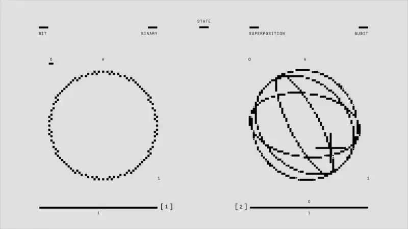
In the ever-accelerating race for computational supremacy, classical machine learning models, despite their impressive advancements, are beginning to brush against fundamental limits. As datasets burgeon in size and complexity, the computational cost of extracting meaningful insights grows exponentially. We’re witnessing the rise of complex, non-linear relationships that even the most sophisticated deep learning architectures struggle to untangle efficiently. This inflection point heralds the arrival of an entirely new paradigm: Quantum Machine Learning (QML). Not merely an incremental upgrade, QML represents a profound architectural shift, leveraging the counter-intuitive yet powerful principles of quantum mechanics—superposition, entanglement, and quantum interference—to process information in ways fundamentally impossible for classical computers.

This isn’t speculative fiction; it’s the bleeding edge of academic research transitioning rapidly into practical development. From arXiv preprints detailing novel quantum kernel methods to GitHub repositories showcasing open-source QML frameworks like Qiskit, Cirq, and PennyLane, the foundations are being laid. TechCrunch and Y Combinator reports increasingly highlight startups pushing the boundaries of quantum algorithms, attracting significant investment. QML promises to unlock unprecedented capabilities in areas ranging from drug discovery and materials science to financial modeling and advanced artificial intelligence, potentially solving problems currently intractable for even the world’s most powerful supercomputers. This article will delve into the technical underpinnings, key algorithms, hybrid architectures, and the practical tools shaping this thrilling new frontier, providing a roadmap for data scientists ready to embark on the quantum journey.

The Quantum Leap in Data Representation: Qubits and Feature Maps

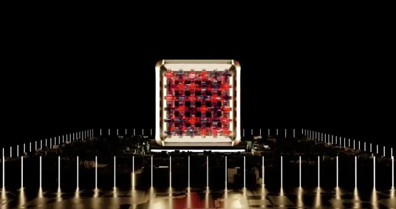
At the core of Quantum Machine Learning lies a radical departure from classical data representation. While classical bits exist in a definite state of 0 or 1, quantum bits, or qubits, can exist in a superposition of both states simultaneously. This inherent probabilistic nature, combined with entanglement—where qubits become correlated in a way that transcends classical physics—allows for an exponential increase in the information density and processing power of a quantum system. A system of n qubits can represent 2^n states concurrently, a phenomenon that provides the quantum advantage for certain types of computations.

The critical first step in applying quantum algorithms to classical machine learning problems is transforming classical data into quantum states. This is achieved through Quantum Feature Maps (QFMs). A QFM is essentially a parametrized quantum circuit that encodes classical input data points x into a high-dimensional quantum Hilbert space, typically by applying a series of quantum gates controlled by the input features. The goal is to map data in such a way that patterns and relationships that are obscure in classical space become more separable or distinguishable in the quantum space, often making linear separations possible in an exponentially larger feature space. This is analogous to the “kernel trick” in classical Support Vector Machines (SVMs), but with the potential to explore feature spaces of vastly greater dimensions. The choice of QFM is crucial, as an inappropriate mapping can lead to issues like “barren plateaus” in variational algorithms, where gradients vanish, hindering optimization.

Consider a simple quantum feature map implemented using Qiskit. This map might involve applying single-qubit rotations (like R_x, R_y, R_z) and entangling gates (like CNOT) whose parameters are derived from the input data.

import numpy as np
from qiskit import QuantumCircuit, Aer, transpile
from qiskit.opflow import StateFn, PauliSumOp
from qiskit.utils import QuantumInstance
from qiskit.circuit.library import ZZFeatureMap

# 1. Define a classical data point (e.g., 2 features)
x = np.array([0.5, 0.8])

# 2. Choose a Quantum Feature Map. ZZFeatureMap is a common choice.
#    It encodes data using Z-rotations and ZZ-interactions.
#    'reps' parameter controls the depth of the circuit (how many times the pattern repeats).
feature_map = ZZFeatureMap(feature_dimension=len(x), reps=2, entanglement='linear')

# 3. Bind the classical data to the feature map
#    The feature map will use 'x' to set its parameters.
feature_map_circuit = feature_map.assign_parameters(x)

# 4. Visualize the circuit (optional)
# print(feature_map_circuit.decompose())

# 5. Simulate the state prepared by the feature map
simulator = Aer.get_backend('statevector_simulator')
quantum_instance = QuantumInstance(simulator, shots=1024)

# Create a job to run the circuit
job = simulator.run(transpile(feature_map_circuit, simulator))
result = job.result()
statevector = result.get_statevector(feature_map_circuit)

print("Classical Input Data:", x)
print("Quantum Feature Map Circuit Depth:", feature_map_circuit.depth())
print("Quantum State Vector (Magnitude):", np.round(np.abs(statevector), 4))
print("This state vector represents the classical data encoded in a high-dimensional quantum space.")

# For a more complex application, this state could then be fed into a quantum kernel
# or a variational quantum classifier.

This Python snippet demonstrates how classical data x is encoded into a quantum state via a ZZFeatureMap. The resulting state vector exists in a complex Hilbert space, where distances and similarities between data points can be profoundly different from their classical counterparts. This initial encoding step is foundational, setting the stage for subsequent quantum algorithms to operate on these quantum representations of data.

Quantum Enhanced Algorithms: QSVMs and QNNs

Leveraging these quantum feature maps, two prominent classes of algorithms emerge in Quantum Machine Learning: Quantum Support Vector Machines (QSVMs) and Quantum Neural Networks (QNNs). These algorithms aim to harness quantum phenomena to outperform their classical counterparts, particularly in tasks involving complex, high-dimensional data.

Quantum Support Vector Machines (QSVMs) are direct quantum extensions of classical SVMs. The core idea is to replace the classical kernel function, which measures the similarity between data points in a high-dimensional feature space, with a Quantum Kernel. A quantum kernel calculates the inner product between two quantum feature states, $\kappa(x_i, x_j) = |\langle\phi(x_i)|\phi(x_j)\rangle|^2$, where $\phi(x)$ is the quantum state encoded by the feature map from classical data x. This kernel value, estimated by running quantum circuits, is then fed into a classical SVM optimizer. The quantum advantage here stems from the ability of QFMs to implicitly map data into exponentially larger Hilbert spaces than classical kernels can practically achieve, potentially leading to better separation boundaries for non-linearly separable data. However, precisely estimating these kernel values can be computationally intensive and susceptible to quantum noise.

Quantum Neural Networks (QNNs), often referred to as Variational Quantum Circuits (VQCs) or Parametrized Quantum Circuits (PQCs), represent a hybrid quantum-classical approach inspired by classical neural networks. A QNN consists of a parametrized quantum circuit whose gate rotation angles are trainable parameters. The circuit takes classical data (encoded via a QFM) and processes it to produce an output, often an expectation value of a specific observable. This output is then fed into a classical loss function, and a classical optimizer updates the quantum circuit’s parameters based on the gradient of the loss. This iterative process, where quantum hardware performs the forward pass and classical computers handle optimization, is a hallmark of the Noisy Intermediate-Scale Quantum (NISQ) era, where full quantum error correction is not yet available.

A typical QNN might look like a series of interleaved layers of single-qubit rotations and entangling gates, where the rotation angles are the variational parameters. Training these QNNs involves challenges such as barren plateaus, where the landscape of the loss function becomes extremely flat for deep circuits, making gradient-based optimization difficult. Techniques like parameter shift rules are used to calculate gradients on quantum hardware.

Here’s a conceptual Python example demonstrating a simple QNN (VQC) with PennyLane, showing the hybrid optimization loop:

import pennylane as qml
from pennylane import numpy as np
from pennylane.optimize import AdamOptimizer

# 1. Define the quantum device
dev = qml.device("default.qubit", wires=2)

# 2. Define the Parametrized Quantum Circuit (PQC / QNN)
#    This circuit will act as our 'quantum layer'
@qml.qnode(dev)
def qnn(weights, x):
    # Encoding layer (simple example using angles from data)
    qml.RY(x[0], wires=0)
    qml.RX(x[1], wires=1)

    # Variational layer (trainable parameters 'weights')
    qml.Rot(weights[0, 0], weights[0, 1], weights[0, 2], wires=0)
    qml.Rot(weights[1, 0], weights[1, 1], weights[1, 2], wires=1)
    qml.CZ(wires=[0, 1])
    qml.Rot(weights[2, 0], weights[2, 1], weights[2, 2], wires=0)
    qml.Rot(weights[3, 0], weights[3, 1], weights[3, 2], wires=1)

    # Measurement (expectation value for classification)
    return qml.expval(qml.PauliZ(0))

# 3. Define a classical cost function
def cost(weights, X, y):
    predictions = [qnn(weights, x) for x in X]
    # Simple squared error loss
    return np.mean((np.array(predictions) - y)**2)

# 4. Generate some dummy data for demonstration
X = np.array([[0.1, 0.2], [0.3, 0.4], [0.5, 0.6], [0.7, 0.8]], requires_grad=False)
y = np.array([0.0, 0.2, 0.5, 0.8], requires_grad=False) # Target outputs

# 5. Initialize random weights for the QNN
#    Number of weights depends on the circuit architecture (4x3 rotations + 1 CZ)
weights = np.random.uniform(low=-np.pi, high=np.pi, size=(4, 3), requires_grad=True)

# 6. Set up the classical optimizer
opt = AdamOptimizer(stepsize=0.1)

# 7. Training loop (hybrid quantum-classical optimization)
epochs = 50
print("Initial cost:", cost(weights, X, y))

for epoch in range(epochs):
    weights, current_cost = opt.step_and_cost(cost, weights, X, y)
    if (epoch + 1) % 10 == 0:
        print(f"Epoch {epoch+1}, Cost: {current_cost:.4f}")

print("Optimized weights:", weights)
print("Final cost:", cost(weights, X, y))

This example illustrates the fundamental hybrid approach: the quantum qnn function computes an output based on data and weights, and a classical AdamOptimizer iteratively adjusts these weights to minimize a cost function. This synergy between quantum and classical components is key to near-term QML applications.

Hybrid Quantum-Classical Architectures for Scalability

The current state of quantum hardware, characterized by the NISQ (Noisy Intermediate-Scale Quantum) era, necessitates a hybrid approach to Quantum Machine Learning. Full-scale, fault-tolerant quantum computers are still years away. Therefore, for practical applications, QML algorithms often involve a delicate dance between quantum processors (QPUs) and classical computing resources. This hybrid architecture is not a temporary workaround but a fundamental paradigm for leveraging the nascent power of QPUs.

In a hybrid setup, the computationally intensive parts that benefit from quantum mechanics (e.g., preparing complex quantum states, executing quantum kernels, performing specific unitary transformations) are offloaded to a QPU. Meanwhile, classical computers handle tasks like data pre-processing, post-processing, optimization of quantum circuit parameters, and overall control flow. This modular design allows researchers to tackle problems too complex for classical machines alone while circumventing the limitations of current noisy quantum hardware.

Key hybrid algorithms include:

• Variational Quantum Eigensolver (VQE): Primarily used in quantum chemistry for finding the ground state energy of molecules. A QPU prepares an ansatz state, measures its energy, and a classical optimizer iteratively adjusts the ansatz parameters to minimize the energy.
• Quantum Approximate Optimization Algorithm (QAOA): Designed for combinatorial optimization problems. Similar to VQE, it uses a parametrized quantum circuit to explore solution spaces and a classical optimizer to find optimal parameters.

The interaction between the classical and quantum components often involves a feedback loop:

1. Classical Pre-processing: Prepare classical data, design the quantum circuit structure (ansatz).
2. Data Encoding: Map classical data to quantum states on the QPU.
3. Quantum Circuit Execution: Run the parametrized quantum circuit on the QPU. This generates quantum measurements.
4. Classical Measurement Post-processing: Extract expectation values or probabilities from quantum measurements.
5. Classical Optimization: Use the extracted values in a classical cost function and update the quantum circuit’s parameters (e.g., gate rotation angles) using classical optimization algorithms (like Adam, L-BFGS-B).
6. Iteration: Send the updated parameters back to the QPU for the next iteration.

One of the significant challenges in these architectures is the data transfer bottleneck between classical and quantum systems, as well as managing error accumulation on noisy QPUs. Techniques like measurement error mitigation and readout error correction are crucial.

Consider a conceptual Bash script that outlines a workflow for running a QML experiment, demonstrating the interplay:

#!/bin/bash

# This script simulates a hybrid quantum-classical workflow.
# It assumes you have a Python environment set up with Qiskit/PennyLane.

echo "Starting Hybrid Quantum-Classical QML Experiment..."

# --- Phase 1: Classical Data Preprocessing ---
echo "1. Performing classical data preprocessing..."
python -c "
import numpy as np
# Simulate loading and cleaning data
data = np.random.rand(100, 2)
labels = (np.sum(data, axis=1) > 1.0).astype(int)
np.save('processed_data.npy', data)
np.save('processed_labels.npy', labels)
print('Data preprocessed and saved to processed_data.npy and processed_labels.npy')
"
echo "Data preprocessing complete."

# --- Phase 2: Initialize Quantum Circuit Parameters Classically ---
echo "2. Initializing quantum circuit parameters..."
python -c "
import numpy as np
# For a variational quantum circuit, we need initial random weights
initial_weights = np.random.uniform(low=-np.pi, high=np.pi, size=(10,)) # Example: 10 parameters
np.save('initial_q_weights.npy', initial_weights)
print('Initial quantum weights saved to initial_q_weights.npy')
"
echo "Quantum circuit parameters initialized."

# --- Phase 3: Hybrid Optimization Loop ---
echo "3. Entering hybrid optimization loop (simulated for simplicity)..."
MAX_ITERATIONS=5

for i in $(seq 1 $MAX_ITERATIONS); do
    echo "--- Iteration $i ---"

    # Classical side prepares data and current weights for quantum execution
    # Quantum side executes the VQC and returns expectation values
    python -c "
    import numpy as np
    # Load processed data and current weights
    data = np.load('processed_data.npy')
    labels = np.load('processed_labels.npy')
    current_weights = np.load('initial_q_weights.npy') if $i == 1 else np.load('optimized_q_weights.npy')

    # Simulate running a QML model (e.g., a QNN) on a QPU
    # In a real scenario, this would involve sending jobs to IBM Quantum, AWS Braket, etc.
    # For now, we simulate a simple cost evaluation
    simulated_quantum_cost = np.mean(np.sin(data @ current_weights[:2] + current_weights[2])**2 - labels)
    print(f'   Simulated Quantum Cost from QPU: {simulated_quantum_cost:.4f}')

    # Classical optimizer computes gradients and updates weights
    # This is where a classical ML framework (e.g., PyTorch, JAX) would interact with quantum backends
    # Simulate a simple gradient update
    learning_rate = 0.05
    gradient_approximation = np.random.rand(current_weights.shape[0]) * 0.1 # Placeholder for actual gradient
    new_weights = current_weights - learning_rate * gradient_approximation
    np.save('optimized_q_weights.npy', new_weights)
    print('   Classical optimizer updated quantum weights.')
    "
done

echo "Hybrid optimization loop complete. Final weights saved to optimized_q_weights.npy."

# --- Phase 4: Classical Post-processing and Evaluation ---
echo "4. Performing classical post-processing and evaluation..."
python -c "
import numpy as np
final_weights = np.load('optimized_q_weights.npy')
# Load a test dataset (not done in this simple script for brevity)
# Evaluate the QML model's performance using the final weights
# print('Final model predictions and performance metrics...')
print('Final weights for deployment:', final_weights)
"
echo "Experiment finished."

This Bash script illustrates a conceptual flow, where Python scripts simulate different stages of the hybrid process, including data handling, parameter initialization, a simulated quantum-classical optimization loop, and final evaluation. This workflow highlights the modularity and iterative nature essential for current QML research.

---

👉 Continue Reading: Unlocking the Quantum Epoch: How QML Will Revolutionize Data Science and AI as We Know It (Part 2)

---

#QuantumMachineLearning #QML #QuantumComputing #DataScience #AI