The Robotics & Autonomous Systems Engineer: Architecting the Future of Intelligent Machines

The Silent Revolution: How Robotics & Autonomous Systems Engineers Are Redefining Intelligence

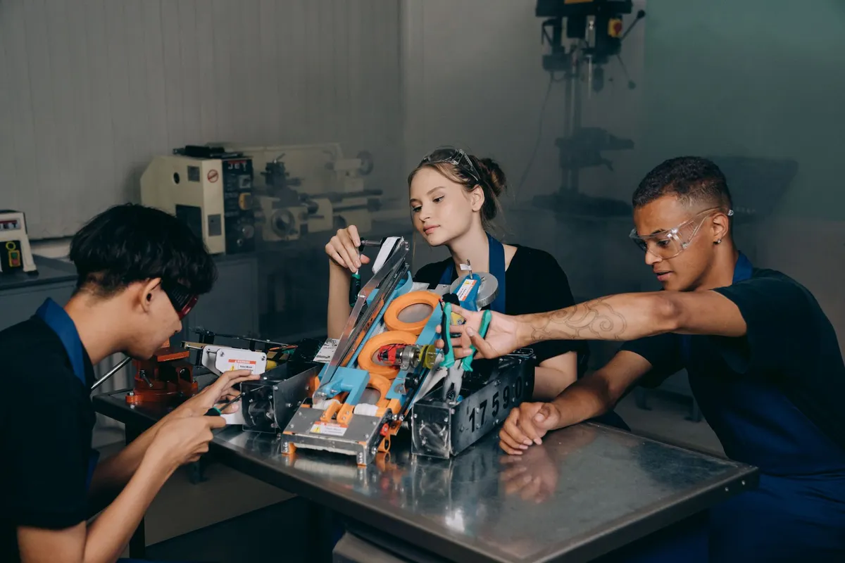
The robotics engineer of 2026 is not just a builder of machines—they are the architects of a new cognitive frontier. From self-driving cars navigating urban jungles to surgical robots performing life-saving operations with sub-millimeter precision, autonomous systems are no longer science fiction. They are the backbone of modern industry, healthcare, and exploration. At the heart of this transformation lies the Robotics & Autonomous Systems Engineer—a multidisciplinary virtuoso who fuses deep mathematical insight, real-time control theory, and adaptive learning into systems that perceive, decide, and act with near-human (and often superhuman) capability.

This role demands more than technical prowess; it requires a philosophical understanding of autonomy itself. What does it mean for a machine to “learn”? How do we ensure safety when a robot’s decision could mean the difference between life and death? And how do we scale intelligence across distributed, heterogeneous systems?

To answer these questions, we must go beyond the surface. We’ll dissect the mathematical foundations of autonomous behavior, explore the latest frameworks enabling self-improving agents, and examine the engineering realities of deploying intelligent systems in the real world. Whether you’re an aspiring engineer, a seasoned developer pivoting into robotics, or a leader shaping the next generation of intelligent machines, this guide will illuminate the path forward.

---

The Mathematical Soul of Autonomous Intelligence

At the core of every autonomous system lies a profound interplay between geometry, probability, and dynamics. The recent breakthroughs in Gromov-Wasserstein gradient flows—a geometric framework for comparing and evolving probability distributions—are reshaping how we model learning and adaptation in high-dimensional spaces. These ideas are not abstract curiosities; they underpin modern robotics control, reinforcement learning, and even multi-agent coordination.

From Wasserstein to Gromov: A Geometric Revolution

The Wasserstein distance, rooted in optimal transport theory, measures the minimal “work” required to morph one probability distribution into another. It has become the gold standard for comparing learned policies, state distributions, and even neural network activations. But when we move from flat Euclidean spaces to structured, relational domains—such as graphs, point clouds, or robotic kinematic chains—we need a more expressive tool.

Enter the Gromov-Wasserstein (GW) distance, which compares distributions while preserving their internal geometry. Unlike Wasserstein, GW accounts for the structure of the data. For instance, in robotics, two different robotic arms might have vastly different joint configurations, but if their end-effector trajectories are geometrically similar, GW can recognize that similarity.

Recent work, such as the arXiv paper “Probabilistic Representation and Convergence of Gromov-Wasserstein Gradient Flows”, extends this idea to gradient flows—continuous-time dynamics that minimize an energy functional (like relative entropy) over structured spaces. The authors show that while the relative entropy functional fails to be convex in the standard GW geometry, it exhibits local convexity under certain conditions. This subtle insight allows the construction of well-defined gradient flows that converge to equilibrium—exactly the kind of stability we demand in autonomous systems.

# Simplified Gromov-Wasserstein gradient flow simulation (conceptual)
import numpy as np
from scipy.optimize import minimize

def gromov_wasserstein_gradient_flow(X, Y, mu, nu, steps=100, lr=0.01):
    """
    Simulates a Gromov-Wasserstein gradient flow between two point clouds X and Y
    with distributions mu and nu.
    """
    T = np.random.rand(X.shape[0], Y.shape[0])
    T = T / T.sum(axis=1, keepdims=True)

    for _ in range(steps):
        # Compute cost matrix in feature space
        C_X = np.linalg.norm(X[:, None] - X[None, :], axis=2)
        C_Y = np.linalg.norm(Y[:, None] - Y[None, :], axis=2)
        L = np.einsum('ij,jk,kl->il', T, C_X, T.T) - C_Y

        # Gradient step (simplified)
        grad = 2 * (np.einsum('ik,jl,ij->kl', T, C_X, L) - np.einsum('ik,jl,ij->kl', L, C_Y, T))
        T -= lr * grad
        T = np.clip(T, 1e-6, None)
        T = T / T.sum(axis=1, keepdims=True)

    return T

# Example usage (synthetic data)
X = np.random.randn(50, 2)
Y = X @ np.array([[1, 0.5], [0.5, 1]]) + 0.1 * np.random.randn(50, 2)
mu = np.ones(50) / 50
nu = np.ones(50) / 50

transport_plan = gromov_wasserstein_gradient_flow(X, Y, mu, nu)

This code block is a conceptual simulation. Real implementations use specialized libraries like pot (Python Optimal Transport) or geomloss, which leverage GPU acceleration and entropy regularization for scalability.

From Gradient Flows to Fokker–Planck Dynamics

The paper further derives a nonlinear Fokker–Planck equation from the GW gradient flow. The Fokker–Planck equation describes how a probability density evolves under diffusion and drift—exactly the kind of dynamics we see in robotic state estimation or policy learning.

What’s remarkable is the decoupling of second moments. The authors show that the covariance of the system evolves independently via an autonomous matrix ODE, reducing the full dynamics to a linear, time-inhomogeneous Fokker–Planck equation. This is akin to the Ornstein–Uhlenbeck process—a stochastic process used in finance, physics, and now robotics to model mean-reverting behavior.

# Docker Compose for simulating Fokker-Planck dynamics (JAX-based)
version: '3.8'
services:
  fokker-planck-sim:
    image: nvcr.io/nvidia/jax:latest
    volumes:
      - ./:/app
    working_dir: /app
    command: >
      python -c "
      import jax
      import jax.numpy as jnp
      from jax.scipy.stats import norm
      import matplotlib.pyplot as plt

      # Simulate Ornstein-Uhlenbeck process
      def ou_process(key, x0, theta, sigma, dt, steps):
          def step(carry, _):
              x, key = carry
              key, subkey = jax.random.split(key)
              noise = jax.random.normal(subkey) * jnp.sqrt(dt) * sigma
              dx = -theta * x * dt + noise
              return (x + dx, key), x

          keys = jax.random.split(key, steps)
          _, xs = jax.lax.scan(step, (x0, key), None, length=steps)
          return xs

      key = jax.random.PRNGKey(42)
      x0 = jnp.array([0.0])
      theta = 1.0
      sigma = 0.5
      dt = 0.01
      steps = 1000

      trajectory = ou_process(key, x0, theta, sigma, dt, steps)
      plt.plot(trajectory)
      plt.title('Ornstein-Uhlenbeck Process (JAX)')
      plt.savefig('/app/ou_process.png')
      "
    deploy:
      resources:
        reservations:
          devices:
            - driver: nvidia
              count: 1
              capabilities: [gpu]

This Docker setup uses JAX to simulate the Ornstein–Uhlenbeck process—a foundational model in stochastic control and robotics. The decoupling of moments is crucial for real-time state estimation in autonomous vehicles, where the covariance of the vehicle’s pose must be tracked efficiently.

---

Self-Improving Agents: The Rise of Adaptive Learning Environments

While gradient flows provide the mathematical backbone, self-improving agents are the engines of tomorrow’s autonomous systems. Traditional reinforcement learning (RL) relies on fixed environments—static benchmarks that don’t evolve with the agent. But real-world intelligence demands adaptive challenge.

Enter SPADE (Self-Play in Adaptive Synthetic Executable Environments), a framework that turns the environment itself into a learnable component. Developed by researchers leveraging large language models (LLMs), SPADE enables agents to design their own training grounds, pushing the boundaries of their capabilities through self-play.

How SPADE Works: A Dual-Agent Architecture

SPADE introduces a two-role LLM system:

1. Environment Designer: Writes executable, long-horizon environments in Python (with reset() and step() interfaces), complete with state transitions, reward functions, and verification logic.
2. Reasoning Agent: Learns to act within these environments, optimizing for regret minimization—the gap between its performance with and without privileged hints.

The key innovation is adaptive difficulty scaling. The Environment Designer doesn’t just generate random tasks; it targets the edge of the agent’s competence, ensuring continuous growth without frustration.

# Minimal SPADE-style environment generator (conceptual)
import gym
from gym import spaces
import numpy as np

class AdaptiveMathEnv(gym.Env):
    """A synthetic math environment that adapts difficulty based on agent performance."""
    def __init__(self):
        super().__init__()
        self.action_space = spaces.Discrete(4)  # 0: add, 1: subtract, 2: multiply, 3: divide
        self.observation_space = spaces.Box(low=0, high=100, shape=(2,), dtype=np.float32)
        self.target = 50.0
        self.current = 0.0
        self.difficulty = 1.0  # Scales the range of numbers

    def reset(self):
        self.current = 0.0
        self.difficulty = min(10.0, self.difficulty * 1.1)  # Increase difficulty
        return np.array([self.current, self.target * self.difficulty])

    def step(self, action):
        if action == 0:
            self.current += self.difficulty
        elif action == 1:
            self.current -= self.difficulty
        elif action == 2:
            self.current *= self.difficulty
        elif action == 3:
            if self.difficulty != 0:
                self.current /= self.difficulty

        reward = -abs(self.current - self.target * self.difficulty)
        done = abs(self.current - self.target * self.difficulty) < 1e-2
        return np.array([self.current, self.target * self.difficulty]), reward, done, {}

# Example usage
env = AdaptiveMathEnv()
obs = env.reset()
for _ in range(10):
    action = env.action_space.sample()  # Replace with RL agent
    obs, reward, done, _ = env.step(action)
    print(f"State: {obs}, Reward: {reward:.2f}, Done: {done}")
    if done:
        obs = env.reset()

This toy example illustrates the core idea: the environment adapts in real-time to the agent’s skill level. In the SPADE paper, this principle is scaled to 30B-parameter models, achieving +5.3 average improvement across math, science, and code benchmarks.

Why This Matters for Robotics

Autonomous robots operate in open-ended, unstructured worlds. They cannot rely on curated datasets or fixed training environments. SPADE-style frameworks enable robots to:

• Generate their own training scenarios (e.g., navigating a warehouse with dynamic obstacles).
• Discover novel failure modes and adapt control policies accordingly.
• Achieve open-ended learning, a holy grail in AI.

This approach is already being explored in multi-agent robotics, where robots compete or collaborate in simulated worlds before deployment.

---

The Embedded Intelligence Stack: From Theory to Silicon

Robotic systems are not just software—they are cyber-physical systems where code meets the real world. A Robotics & Autonomous Systems Engineer must master the full stack: from high-level control theory to low-level firmware, from sensor fusion to safety certification.

Real-Time Operating Systems & Middleware

Modern robots run on real-time operating systems (RTOS) like QNX, FreeRTOS, or ROS 2 (with real-time extensions). The latter is particularly dominant in research and industry.

# ROS 2 Docker Compose for a robotic navigation stack
version: '3.8'
services:
  ros2-core:
    image: osrf/ros:humble-desktop-full
    volumes:
      - ./ros2_ws:/root/ros2_ws
    working_dir: /root/ros2_ws
    command: >
      bash -c "
      source /opt/ros/humble/setup.bash &&
      ros2 run demo_nodes_cpp talker
      "
    network_mode: host
    privileged: true
    environment:
      - DISPLAY=$DISPLAY
      - QT_X11_NO_MITSHM=1
    volumes:
      - /tmp/.X11-unix:/tmp/.X11-unix

  ros2-nav:
    image: ros:humble-ros-core
    depends_on:
      - ros2-core
    command: >
      bash -c "
      source /opt/ros/humble/setup.bash &&
      ros2 launch nav2_bringup navigation_launch.py use_sim_time:=True
      "

This setup launches a ROS 2 navigation stack in Docker, simulating a robot navigating an environment. Key components:

• demo_nodes_cpp: Publishes sensor data (simulated).
• nav2_bringup: Handles path planning, obstacle avoidance, and localization.

Sensor Fusion: The Art of Perceiving the World

Autonomous systems rely on sensor fusion to estimate state. Common sensors:

• LiDAR: 3D point clouds for mapping.
• IMU: Accelerometer + gyroscope for orientation.
• Cameras: RGB for object detection (YOLO, Segment Anything Model).
• Radar: For adverse weather conditions.

A typical fusion pipeline uses Kalman Filters (EKF, UKF) or Particle Filters to combine noisy measurements.

# Extended Kalman Filter (EKF) for robot localization (simplified)
import numpy as np
from scipy.linalg import block_diag

class EKFLocalizer:
    def __init__(self, initial_state, initial_covariance, process_noise, measurement_noise):
        self.state = initial_state  # [x, y, theta]
        self.covariance = initial_covariance
        self.Q = process_noise
        self.R = measurement_noise

    def predict(self, control_input, dt):
        # State transition model (bicycle model)
        v, omega = control_input
        theta = self.state[2]
        self.state[0] += v * np.cos(theta) * dt
        self.state[1] += v * np.sin(theta) * dt
        self.state[2] += omega * dt

        # Jacobian of the motion model
        F = np.array([
            [1, 0, -v * np.sin(theta) * dt],
            [0, 1,  v * np.cos(theta) * dt],
            [0, 0, 1]
        ])

        self.covariance = F @ self.covariance @ F.T + self.Q

    def update(self, measurement, H, z_pred):
        # H: Measurement model Jacobian
        # z_pred: Predicted measurement
        y = measurement - z_pred
        S = H @ self.covariance @ H.T + self.R
        K = self.covariance @ H.T @ np.linalg.inv(S)
        self.state = self.state + K @ y
        self.covariance = (np.eye(3) - K @ H) @ self.covariance

# Example usage
ekf = EKFLocalizer(
    initial_state=np.array([0, 0, 0]),
    initial_covariance=np.eye(3) * 0.1,
    process_noise=np.eye(3) * 0.01,
    measurement_noise=np.eye(2) * 0.5
)

# Simulate a robot moving in a circle
for t in range(100):
    control = np.array([1.0, 0.1])  # v, omega
    ekf.predict(control, dt=0.1)
    # Simulate a noisy GPS measurement (x, y)
    measurement = ekf.state[:2] + np.random.randn(2) * 0.3
    H = np.array([[1, 0, 0], [0, 1, 0]])  # Only observe x and y
    ekf.update(measurement, H, ekf.state[:2])
    print(f"Estimated state: {ekf.state}")

This EKF implementation fuses odometry (control input) with GPS-like measurements to estimate a robot’s pose. In practice, engineers use libraries like ROS 2’s robot_localization or Kalman filter implementations in C++ for embedded systems.

---

Safety, Ethics, and the Responsibility of Autonomy

Autonomous systems are not just technical marvels—they are moral artifacts. A misstep in a self-driving car or a surgical robot can have catastrophic consequences. The Robotics & Autonomous Systems Engineer must embed safety, interpretability, and ethical reasoning into every layer of the system.

Formal Methods & Verification

To ensure correctness, engineers use formal methods:

• Model Checking: Verify that a control policy satisfies temporal logic properties (e.g., “The robot never collides”).
• Runtime Monitoring: Use runtime verification to detect deviations from expected behavior.
• Formal Synthesis: Automatically generate control laws that satisfy safety constraints.

Tools like TLA+, UPPAAL, and ROS 2’s safety_lifecycle are gaining traction.

# TLA+ specification for a safe robotic arm (simplified)
---- MODULE SafeArm ----
EXTENDS Naturals, TLC

CONSTANTS MaxAngle, MaxVelocity

VARIABLES current_angle, current_velocity, target_angle

SafeAngle == current_angle <= MaxAngle
SafeVelocity == Abs(current_velocity) <= MaxVelocity

Next ==
    /\ current_angle' = current_angle + current_velocity * dt
    /\ current_velocity' = (target_angle - current_angle) * kp - current_velocity * kd
    /\ SafeAngle
    /\ SafeVelocity

Spec == Init /\ [][Next]_<<current_angle, current_velocity, target_angle>>

THEOREM Spec => []SafeAngle
====

This TLA+ module ensures that a robotic arm never exceeds its maximum angle and velocity limits. Formal methods like this are increasingly required in automotive (ISO 26262) and medical robotics (IEC 62304).

Ethical AI in Robotics

Autonomous systems must make ethical trade-offs. For example:

• A self-driving car must decide between swerving (risking the passenger) or staying in lane (risking pedestrians).
• A surgical robot must prioritize patient safety over procedure speed.

Frameworks like Asimov’s Laws are too simplistic. Instead, engineers use value-sensitive design and participatory design to align systems with human values.

---

The Career Blueprint: Skills, Tools, and Pathways

Becoming a Robotics & Autonomous Systems Engineer requires a diverse skill set and hands-on experience. Here’s a structured pathway:

Core Competencies

Domain	Key Skills	Tools & Frameworks
Control Theory	PID, LQR, MPC, Kalman Filters	MATLAB, ROS 2, CasADi
Machine Learning	Reinforcement Learning, Imitation Learning	PyTorch, JAX, Stable Baselines3
Computer Vision	Object Detection, SLAM, Segmentation	OpenCV, ROS 2 Vision, SAM
Embedded Systems	RTOS, Firmware, Hardware Abstraction	FreeRTOS, Zephyr, Arduino, STM32
Robotics Middleware	ROS 2, MoveIt, Navigation Stack	Docker, Gazebo, Ignition
Safety & Verification	Formal Methods, Runtime Monitoring	TLA+, UPPAAL, ROS 2 Safety

Learning Path

1. Foundations:
   • Linear Algebra (Gilbert Strang)
   • Probability (Dimitri Bertsekas)
   • Control Theory (Richard Murray)
2. Robotics:
   • Modern Robotics (Kevin Lynch)
   • Probabilistic Robotics (Sebastian Thrun)
3. AI/ML:
   • Reinforcement Learning: An Introduction (Sutton & Barto)
   • Deep Learning (Ian Goodfellow)
4. Hands-On:
   • Build a ROS 2 robot (e.g., TurtleBot3).
   • Implement SLAM (ORB-SLAM3).
   • Train a reinforcement learning agent (Stable Baselines3).

Career Trajectories

• Research Engineer: Work at labs (e.g., Boston Dynamics, DeepMind Robotics) or academia.
• Autonomous Vehicle Engineer: Join teams at Tesla, Waymo, or Cruise.
• Medical Robotics Engineer: Develop surgical robots (Intuitive Surgical, Stryker).
• Industrial Automation Engineer: Design robotic arms for manufacturing (ABB, KUKA).
• Entrepreneur: Found a robotics startup (e.g., Figure AI, Agility Robotics).

---

The Future: Toward General Autonomous Intelligence

We are on the cusp of a new era—General Autonomous Intelligence (GAI)—where robots can operate across domains with human-like adaptability. The path forward involves:

• Neurosymbolic Robotics: Combining deep learning with symbolic reasoning for explainability.
• Multi-Modal Learning: Fusing vision, language, and touch for robust perception.
• Self-Supervised Learning: Enabling robots to learn from raw experience without labels.
• Decentralized Autonomy: Swarms of robots coordinating without central control.

The Robotics & Autonomous Systems Engineer of the future will not only build machines but redefine the boundaries of intelligence itself.

---

The Autonomous Horizon: Where Code Meets the World

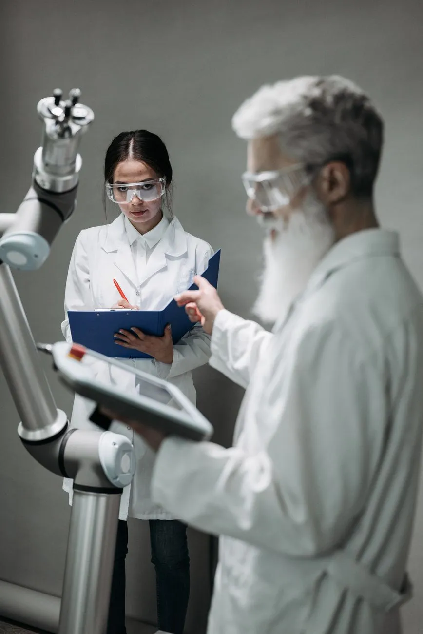
The role of the Robotics & Autonomous Systems Engineer is one of the most challenging, rewarding, and consequential in technology today. It demands a rare blend of mathematical depth, engineering pragmatism, and ethical foresight. From the abstract elegance of Gromov-Wasserstein flows to the gritty reality of deploying a robot in a factory, this field is a testament to human ingenuity.

As autonomous systems permeate every facet of life—from the operating room to the surface of Mars—the engineer who designs them becomes an architect of the future. The tools and theories we’ve explored here are not just academic exercises; they are the blueprints for the next industrial revolution.

The question is no longer can we build autonomous machines. It’s should we—and more importantly, how do we do it right? The answer lies in the hands of the next generation of Robotics & Autonomous Systems Engineers.

---

#RoboticsEngineer #AutonomousSystems #AIinRobotics #EmbeddedAI #ReinforcementLearning #RoboticsCareer #FutureOfAutonomy

Related Insights

• The Haptic Renaissance: How Quantum-Entangled Feedback is Reshaping Remote Surgery
• Mind Meld: Unlocking the Potential of Brain-Computer Interfaces
• Quantum Sensing: The Subatomic Microscope Reshaping Mineral Exploration